From Data to Clinic: A 2025 Guide to Machine Learning for Predictive Biomarker Validation

Abstract

This article provides a comprehensive guide for researchers and drug development professionals on the application of machine learning (ML) in the validation of predictive biomarkers. It covers the foundational principles of biomarkers and their role in precision medicine, explores advanced ML methodologies for biomarker analysis, addresses critical challenges and optimization strategies, and establishes robust frameworks for clinical validation and model comparison. By synthesizing the latest 2025 research and trends, this resource aims to bridge the gap between computational discovery and clinically actionable, validated biomarkers, ultimately accelerating the development of personalized therapeutics.

The New Frontier: Defining Predictive Biomarkers and the Machine Learning Revolution

Biomarkers, defined as "a defined characteristic that is measured as an indicator of normal biological processes, pathogenic processes or responses to an exposure or intervention," form the cornerstone of modern diagnostic and therapeutic development [1]. These measurable indicators appear in blood, tissue, or other biological samples, providing crucial data about normal processes, disease states, and treatment responses [2]. The joint FDA-NIH Biomarkers, EndpointS, and other Tools (BEST) resource has established standardized definitions to create a shared understanding across research and clinical practice, recognizing that confusion about fundamental definitions and concepts has historically slowed progress in diagnostic and therapeutic technology development [1].

The evolution of biomarkers represents a journey from single-molecule measurements to complex multi-omics profiles, reshaping how researchers approach disease understanding and drug development. This transformation is particularly evident in complex fields like chronic disease and nutrition, where single biomarkers often fail to capture disease complexity [1]. The emergence of large-scale biobanks integrating electronic health records with multi-omics data has created unprecedented opportunities to discover novel biomarkers and develop predictive algorithms for human disease [3]. This guide provides a comprehensive comparison of traditional and modern biomarker approaches, examining their performance characteristics, validation methodologies, and applications in contemporary research and drug development.

Traditional Biomarker Classifications and Applications

Fundamental Biomarker Categories

Traditional biomarker classification systems categorize these molecular indicators based on their specific clinical applications and contextual use. The BEST resource defines several critical subtypes with distinct purposes [1]:

• Diagnostic biomarkers detect or confirm the presence of a disease or condition of interest, or identify individuals with a disease subtype. Examples include troponin for myocardial infarction and PSA for prostate cancer screening [1] [2].
• Monitoring biomarkers are measured serially to assess the status of a disease or medical condition, such as hemoglobin A1c in diabetes management or CD4 counts in HIV infection monitoring [1].
• Pharmacodynamic/response biomarkers indicate that a biological response has occurred in an individual who has been exposed to a medical product or environmental agent.
• Predictive biomarkers help identify individuals who are more likely to experience a favorable or unfavorable effect from a specific medical product, enabling targeted therapies.
• Prognostic biomarkers forecast the likelihood of future clinical events, disease recurrence, or progression in patients with a specific medical condition.
• Safety biomarkers are measured before or after exposure to a medical product to indicate the likelihood, presence, or extent of toxicity as an adverse effect.
• Susceptibility/risk biomarkers indicate the potential for developing a disease or medical condition in individuals without clinically apparent disease.

A single biomarker may fulfill multiple roles across different contexts, but each specific use requires separate evidence development and validation [1]. This classification system enables healthcare teams to develop targeted, effective treatment strategies and provides a framework for regulatory evaluation [2].

Comparison of Traditional Biomarker Types

Table 1: Classification and Applications of Traditional Biomarker Types

Biomarker Type	Primary Function	Clinical Context	Examples	Regulatory Considerations
Diagnostic	Detects or confirms disease presence	Identification of disease or subtype	Troponin (myocardial infarction), PSA (prostate cancer)	Must have very low false-positive rate for low-prevalence diseases requiring invasive follow-up [1]
Monitoring	Assesses disease status over time	Serial measurement of disease progression or treatment response	Hemoglobin A1c (diabetes), CD4 counts (HIV)	Optimal measurement intervals and clinical decision thresholds often require refinement [1]
Predictive	Identifies likely treatment responders	Patient stratification for targeted therapies	EGFR mutations (lung cancer), HER2 status (breast cancer)	Critical for enrichment strategies in clinical trials [2]
Prognostic	Forecasts disease course	Informs long-term treatment planning and patient counseling	Cancer staging, Oncotype DX recurrence score	Must be distinguished from predictive biomarkers for proper clinical application [1]
Safety	Indicates potential toxicity	Monitoring adverse effects of treatments	Liver enzymes for hepatotoxicity, QTc prolongation	Often used in early clinical development to identify dose-limiting toxicities [1]

Validation Framework for Traditional Biomarkers

The validation of traditional biomarkers requires a rigorous, multi-step process specific to each condition of use. This process encompasses three interdependent components: analytical validation, qualification using an evidentiary assessment, and utilization [1]. Analytical validation ensures the biomarker can be measured accurately, reliably, and reproducibly through defined analytical methods. Qualification involves assessing the evidence linking the biomarker to a specific biological process or clinical endpoint. Utilization establishes the appropriateness of the biomarker for a specific context in drug development or regulatory decision-making.

The operating characteristics of biomarker assays vary considerably, creating challenges for clinical implementation. For example, the many troponin assays demonstrate substantial variability, especially at lower detection limits where misclassification can significantly impact medical care [1]. The advent of high-sensitivity troponin assays has enabled sophisticated diagnosis of small myocardial necrosis episodes but has simultaneously created new interpretation challenges when elevations occur at previously undetectable levels [1].

The Multi-Omics Revolution in Biomarker Discovery

Multi-Omics Technologies and Their Applications

Multi-omics strategies integrate large-scale, high-throughput analyses across multiple molecular layers, including genomics, transcriptomics, proteomics, metabolomics, and epigenomics [4]. This comprehensive approach provides unprecedented insights into cellular dynamics and facilitates biomarker identification crucial for cancer diagnosis, prognosis, and therapeutic decision-making [4]. Landmark projects such as The Cancer Genome Atlas (TCGA) Pan-Cancer Atlas, the Pan-Cancer Analysis of Whole Genomes (PCAWG), MSK-IMPACT, and the Clinical Proteomic Tumor Analysis Consortium (CPTAC) have demonstrated the utility of multi-omics in uncovering cancer biology and clinically actionable biomarkers [4].

Each omics layer provides distinct biological insights:

• Genomics investigates alterations at the DNA level using sequencing technologies to identify copy number variations, genetic mutations, and single nucleotide polymorphisms [4]. The tumor mutational burden (TMB), validated in the KEYNOTE-158 trial, has been approved by the FDA as a predictive biomarker for pembrolizumab treatment across solid tumors [4].
• Transcriptomics explores RNA expression using microarrays and RNA sequencing, encompassing mRNAs and noncoding RNAs [4]. Clinically validated gene-expression signatures such as Oncotype DX (21-gene) and MammaPrint (70-gene) have demonstrated utility in tailoring adjuvant chemotherapy decisions in breast cancer patients [4].
• Proteomics investigates protein abundance, modifications, and interactions using high-throughput methods including mass spectrometry [4]. CPTAC studies of ovarian and breast cancers showed that proteomics can identify functional subtypes and reveal druggable vulnerabilities missed by genomics alone [4].
• Metabolomics examines cellular metabolites, including small molecules, carbohydrates, lipids, and nucleosides [4]. In IDH1/2-mutant gliomas, the oncometabolite 2-hydroxyglutarate (2-HG) functions as both a diagnostic and mechanistic biomarker [4].
• Epigenomics investigates DNA and histone modifications, including DNA methylation [4]. MGMT promoter methylation serves as a classic clinical biomarker predicting benefit from temozolomide chemotherapy in glioblastoma [4].

Comparative Performance of Multi-Omics Platforms

Table 2: Performance Characteristics of Multi-Omics Technologies in Biomarker Discovery

Omics Layer	Analytical Platforms	Key Biomarker Applications	Clinical Validation Examples	Strengths	Limitations
Genomics	Whole exome sequencing, Whole genome sequencing	Tumor mutational burden, MSI status, BRCA mutations	FDA approval of TMB for pembrolizumab; ~37% of tumors harbor actionable alterations in MSK-IMPACT [4]	Comprehensive mutation profiling; established clinical utility	Does not capture functional protein or regulatory effects
Transcriptomics	RNA sequencing, Microarrays	Gene expression signatures, Fusion genes, Immune signatures	Oncotype DX (TAILORx trial), MammaPrint (MINDACT trial) for breast cancer chemotherapy decisions [4]	High sensitivity and cost-effectiveness; reflects active biological processes	mRNA levels may not correlate with protein abundance
Proteomics	Mass spectrometry, Liquid chromatography-MS	Protein abundance, Post-translational modifications, Pathway activation	CPTAC studies identifying functional subtypes in ovarian and breast cancers [4]	Directly measures functional effectors; post-translational modifications	Analytical complexity; dynamic range challenges
Metabolomics	LC-MS, GC-MS	Metabolic pathway alterations, Oncometabolites	2-hydroxyglutarate in IDH-mutant gliomas; 10-metabolite plasma signature in gastric cancer [4]	Closest to phenotypic expression; dynamic response indicators	Complex sample preparation; database limitations
Epigenomics	Whole genome bisulfite sequencing, ChIP-seq	DNA methylation signatures, Histone modifications	MGMT promoter methylation in glioblastoma; multi-cancer early detection assays [4]	Stable markers; tissue-of-origin signatures	Tissue-specific patterns; complex data interpretation

Experimental Protocols for Multi-Omics Integration

Multi-omics integration involves comprehensive analysis of data from various sources, offering more robust results for biomarker discovery. Two primary integration strategies have emerged [4]:

• Horizontal integration combines the same type of omics data from multiple studies or cohorts to increase statistical power and validate findings across diverse populations.
• Vertical integration simultaneously analyzes different omics layers from the same samples to build comprehensive molecular networks and identify cross-omics interactions.

The experimental workflow for multi-omics biomarker discovery typically includes [4]:

• Sample preparation using standardized protocols for nucleic acid, protein, and metabolite extraction
• Data generation across multiple analytical platforms
• Quality control and normalization within each omics dataset
• Data integration using computational methods
• Biomarker identification and validation in independent cohorts

Quality control steps are critical for each omics data type. For genomics and transcriptomics, this includes assessing sequencing depth, mapping rates, and batch effects. For proteomics, quality metrics encompass peptide identification confidence, protein inference, and quantification accuracy. Metabolomics requires evaluation of peak detection, alignment, and identification reliability [4].

Machine Learning and Computational Frameworks for Biomarker Validation

Advanced Machine Learning Approaches

Machine learning holds significant promise for accelerating biomarker discovery in clinical proteomics and other multi-omics fields, though its real-world impact remains limited by methodological pitfalls and unrealistic expectations [5]. Machine learning enhances biomarker discovery by integrating diverse and high-volume data types, such as genomics, transcriptomics, proteomics, metabolomics, imaging, and clinical records [6]. These approaches successfully identify diagnostic, prognostic, and predictive biomarkers across fields including oncology, infectious diseases, neurological disorders, and autoimmune diseases [6].

Key machine learning methodologies in biomarker discovery include [6]:

• Supervised learning trains predictive models on labeled datasets to classify disease status or predict clinical outcomes using techniques like support vector machines, random forests, and gradient boosting algorithms (XGBoost, LightGBM).
• Unsupervised learning explores unlabeled datasets to discover inherent structures or novel subgroupings without predefined outcomes using clustering methods (k-means, hierarchical clustering) and dimensionality reduction approaches (principal component analysis).
• Deep learning architectures, particularly convolutional neural networks (CNNs) and recurrent neural networks (RNNs), handle complex biomedical data. CNNs identify spatial patterns in imaging data, while RNNs capture temporal dynamics in longitudinal data.

The MILTON framework (machine learning with phenotype associations) exemplifies advanced machine learning applications, utilizing a range of biomarkers to predict 3,213 diseases in the UK Biobank [3]. This ensemble machine-learning framework leverages longitudinal health record data to predict incident disease cases undiagnosed at time of recruitment, largely outperforming available polygenic risk scores [3]. MILTON achieved AUC ≥ 0.7 for 1,091 disease codes, AUC ≥ 0.8 for 384 codes, and AUC ≥ 0.9 for 121 codes across all time-models and ancestries [3].

Experimental Protocol for Machine Learning Validation

Robust machine learning validation requires rigorous methodology to avoid common pitfalls such as overfitting, data leakage, and poor generalizability. A standardized protocol includes [5] [3]:

• Feature Selection: Initial biomarker candidates are identified from multi-omics measurements. Dimensionality reduction techniques may be applied to address the high dimensionality typical of omics data.

• Model Training: Using a training subset (typically 70-80% of data), models are trained with careful attention to avoiding overfitting through techniques like regularization and cross-validation.

• Hyperparameter Tuning: Model parameters are optimized using validation sets or nested cross-validation to maximize performance while maintaining generalizability.

• Performance Evaluation: Models are tested on held-out test sets using appropriate metrics including area under the curve (AUC), sensitivity, specificity, and positive predictive value.

• External Validation: Ideally, models should be validated using completely independent cohorts to assess true generalizability across different populations and settings.

For clinical proteomics specifically, researchers caution against the uncritical application of complex models such as deep learning architectures that often exacerbate problems with small sample sizes, offering limited interpretability and negligible performance gains [5]. Instead, they advocate for realistic and responsible use of machine learning, grounded in rigorous study design, appropriate validation strategies, and transparent, reproducible modeling practices [5].

Biomarker Validation and Comparison Frameworks

Standardized statistical frameworks enable direct comparison of biomarker performance across modalities and measurement techniques. These frameworks operationalize specific criteria including precision in capturing change over time and clinical validity [7]. In Alzheimer's disease research, for example, ventricular volume and hippocampal volume showed the best precision in detecting change over time in both individuals with mild cognitive impairment and dementia [7].

The Biomarker Toolkit provides an evidence-based guideline to predict cancer biomarker success and guide development [8]. Developed through systematic literature review, expert interviews, and Delphi surveys, this validated checklist includes 129 attributes grouped into four main categories: rationale, clinical utility, analytical validity, and clinical validity [8]. Validation studies demonstrated that the total score generated by this toolkit significantly predicts biomarker implementation success in both breast and colorectal cancer [8].

Key validation criteria for biomarkers include [7] [8]:

• Analytical validity: Measures how accurately and reliably the biomarker can be measured, including sensitivity, specificity, reproducibility, and stability.
• Clinical validity: Assesses how accurately the biomarker identifies or predicts the clinical outcome of interest, including prognostic and predictive value.
• Clinical utility: Determines whether using the biomarker for decision-making leads to improved patient outcomes and whether the benefits outweigh any risks or costs.

Visualization and Interpretation of Complex Biomarker Data

Advanced Visualization Techniques

Biomarker heatmaps with clustering analysis enable visualization of complex multi-dimensional biomarker data, helping to identify patterns or trends in relative abundance variations [9]. This approach is particularly valuable for interpreting high-temporal resolution biomarker data, such as monitoring storm-induced changes in fluvial particulate organic carbon composition [9]. The methodology involves:

• Data Scaling: Biomarker concentration data are converted to z-scores using autoscaling to avoid inadvertent weighting due to extreme high or low absolute concentrations.
• Heatmap Construction: Z-scores are visualized using color gradients, with red typically indicating higher-than-average concentrations and blue indicating lower-than-average concentrations.
• Hierarchical Clustering: Both rows and columns are reordered based on similarity in biomarker profiles, grouping similar samples and similar biomarkers together.

This visualization approach helps identify hidden patterns in complex biomarker data and generates hypotheses for follow-up analyses [9]. Compared to principal component analysis (PCA), biomarker heatmaps perform better in visualizing temporal changes of individual biomarkers while maintaining the ability to identify sample clusters [9].

Visualizing Biomarker Classification and Validation Pathways

Diagram 1: Comprehensive Biomarker Discovery and Validation Workflow. This workflow illustrates the pathway from sample collection through multi-omics data generation, computational analysis, classification, and validation to clinical application.

Diagram 2: Multi-Omics Integration for Biomarker Discovery. This diagram shows how different molecular layers are derived from biological samples and integrated to identify comprehensive biomarker signatures.

Key Research Reagent Solutions

Table 3: Essential Research Reagents and Platforms for Biomarker Discovery and Validation

Category	Specific Tools/Reagents	Primary Function	Application Context	Considerations
Sample Preparation	Omni LH 96 homogenizer, Automated nucleic acid extractors	Standardized sample processing and nucleic acid extraction	Critical for reproducible multi-omics studies; reduces human error and processing variability [2]	Automation ensures consistent extraction across studies, reducing variability that compromises analyses [2]
Genomics Platforms	Next-generation sequencers (Illumina), Whole exome/genome kits	Comprehensive DNA mutation and variation profiling	Identification of genetic biomarkers, tumor mutational burden, copy number variations [4]	Library preparation consistency is crucial for comparative analyses; requires rigorous quality control metrics
Proteomics Reagents	Mass spectrometry systems, Antibody arrays, LC-MS platforms	Protein identification, quantification, and post-translational modification mapping	Discovery of protein biomarkers, pathway activation analysis, therapeutic target identification [4] [5]	Standardized protocols essential for cross-study comparisons; dynamic range limitations require consideration
Metabolomics Tools	LC-MS, GC-MS systems, Metabolite standards, Extraction kits	Comprehensive metabolite profiling and quantification	Identification of metabolic biomarkers, pathway analysis, therapeutic response monitoring [4]	Sample stability critical; comprehensive standards libraries needed for compound identification
Computational Resources	Multi-omics databases (TCGA, CPTAC), Machine learning libraries	Data integration, analysis, and biomarker model development	Multi-omics integration, biomarker signature identification, predictive model building [4] [3]	Data harmonization essential; computational expertise required for advanced machine learning applications

The evolution from traditional single-molecule biomarkers to modern multi-omics profiles represents a paradigm shift in diagnostic and therapeutic development. While traditional biomarkers continue to provide critical clinical value in specific contexts, multi-omics approaches offer unprecedented comprehensive profiling of biological systems. The integration of machine learning and computational frameworks enables researchers to extract meaningful patterns from these complex datasets, accelerating biomarker discovery and validation.

Successful biomarker development requires rigorous attention to analytical validation, clinical validity, and demonstrated clinical utility. Frameworks like the Biomarker Toolkit provide evidence-based guidance for prioritizing biomarker development efforts [8]. As multi-omics technologies continue to advance and computational methods become more sophisticated, the biomarker landscape will increasingly embrace complex composite biomarkers and digital biomarkers derived from sensors and mobile technologies [1].

The future of biomarker research lies in effectively integrating traditional clinical knowledge with cutting-edge multi-omics profiling, leveraging machine learning to identify robust signatures, and applying rigorous validation frameworks to ensure clinical utility. This integrated approach promises to deliver more precise, personalized diagnostic and therapeutic strategies, ultimately improving patient outcomes across diverse disease areas.

The Critical Role of Predictive Biomarkers in Precision Medicine and Drug Development

Predictive biomarkers are fundamentally reshaping precision medicine and drug development by enabling patient stratification, forecasting therapeutic efficacy, and guiding targeted treatment strategies. These measurable indicators of biological processes or drug responses have evolved from single-molecule entities to complex multi-analyte signatures, thanks to technological advancements in high-throughput omics profiling and sophisticated computational approaches [10]. The traditional model of "one mutation, one target, one test" is rapidly giving way to multidimensional perspectives that capture the full complexity of disease biology [10]. This paradigm shift is critically supported by machine learning (ML) and artificial intelligence (AI), which can analyze large, complex datasets to identify reliable and clinically useful biomarkers from diverse biological layers including genomics, transcriptomics, proteomics, metabolomics, and digital pathology [6]. The integration of these technologies addresses significant limitations of conventional biomarker discovery methods, including limited reproducibility, high false-positive rates, and inadequate predictive accuracy, ultimately accelerating the development of personalized treatment strategies that maximize therapeutic benefits while minimizing adverse effects [6].

Technological Landscape: Multi-Omics and Machine Learning Integration

Multi-Omics as the Engine of Discovery

The contemporary biomarker discovery landscape is dominated by integrated multi-omics approaches that provide a comprehensive view of disease biology. Spatial biology, single-cell analysis, and multi-omics have transitioned from buzzwords to the fundamental backbone of precision medicine, enabling researchers to move beyond static endpoints and capture dynamic disease processes [10]. Leading technology providers are demonstrating how these approaches reveal clinically actionable insights that traditional methods miss. For instance, 10x Genomics showcased how protein profiling identified tumor regions expressing poor-prognosis biomarkers with known therapeutic targets—signals that standard RNA analysis had entirely missed [10]. Similarly, Element Biosciences' AVITI24 system collapses previously separate workflows by combining sequencing with cell profiling to capture RNA, protein, and morphological data simultaneously [10]. These technological advances enable pharmaceutical companies to transform biomarker-driven drug development and meaningfully improve patient outcomes through more precise patient stratification that considers the full molecular and cellular context of disease rather than single mutations alone [10].

Machine Learning and AI Methodologies

Machine learning enhances biomarker discovery by integrating diverse and high-volume data types to identify diagnostic, prognostic, and predictive biomarkers across various disease areas including oncology, infectious diseases, and neurological disorders [6]. Several methodological approaches have proven particularly effective:

• Supervised Learning Techniques: Include support vector machines (effective for small sample, high-dimensional omics data), random forests (providing robustness against noise and overfitting), and gradient boosting algorithms (e.g., XGBoost, LightGBM) that iteratively correct prediction errors for superior accuracy [6].

• Deep Learning Architectures: Convolutional Neural Networks (CNNs) identify spatial patterns in imaging data such as histopathology, while Recurrent Neural Networks (RNNs) capture temporal dynamics and dependencies within sequential data, making them valuable for prognosis and treatment response prediction [6].

• Automated ML Workflows: Cloud-based platforms like BiomarkerML provide standardized, user-friendly interfaces that streamline analyses and ensure reproducibility. These workflows employ techniques like weighted, nested cross-validation to avoid model over-fitting and data leakage, while using SHapley Additive exPlanations (SHAP) to quantify each protein's contribution to model predictions [11].

The application of these ML methods has demonstrated significant performance improvements over traditional approaches. Research on gastric cancer datasets showed that when specificity was fixed at 0.9, ML approaches achieved a sensitivity of 0.240 with 3 biomarkers and 0.520 with 10 biomarkers, substantially outperforming standard logistic regression which provided sensitivities of 0.000 and 0.040 respectively [12].

Table 1: Comparison of Machine Learning Performance in Biomarker Discovery

Method	Number of Biomarkers	Sensitivity	Specificity	Application Domain
ML Approaches	3	0.240	0.900	Gastric Cancer
ML Approaches	10	0.520	0.900	Gastric Cancer
Logistic Regression	3	0.000	0.900	Gastric Cancer
Logistic Regression	10	0.040	0.900	Gastric Cancer
Random Forest Classifier	Digital Biomarkers	0.882	0.841	Alzheimer's Disease
BiomarkerML Workflow	Proteomic Features	Varies by dataset	Varies by dataset	Multi-Disease Application

Experimental Approaches and Validation Frameworks

Methodologies for Biomarker Discovery and Validation

Robust experimental protocols are essential for translating biomarker discoveries into clinically applicable tools. The following methodologies represent current best practices across different biomarker types:

Proteomic Biomarker Discovery Using BiomarkerML The BiomarkerML workflow provides a comprehensive framework for proteomic biomarker discovery [11]. The process begins with data ingestion of proteomic and clinical data alongside sample labels. Subsequent pre-processing prepares data for model fitting, with optional dimensionality reduction and visualization. The workflow then fits a catalog of ML and DL classification and regression models, calculating performance metrics for model comparison. A critical step involves applying mean SHapley Additive exPlanations (SHAP) to quantify the contribution of each protein to model predictions across all samples. Proteins with high mean SHAP values and their co-expressed protein network interactors are finally identified as candidate biomarkers. This workflow employs hyperparameter fine-tuning via grid-search and weighted, nested cross-validation to prevent model over-fitting and data leakage, ensuring reproducible results [11].

Blood-Based Digital Biomarkers for Alzheimer's Disease A multicohort diagnostic study demonstrated an innovative approach for developing ML models with blood-based digital biomarkers for Alzheimer's disease diagnosis [13]. Researchers used Attenuated Total Reflectance-Fourier Transform Infrared (ATR-FTIR) spectroscopy to generate plasma spectra data from 1324 individuals, including patients with Alzheimer's disease, mild cognitive impairment, and other neurodegenerative diseases. They applied random forest classifiers with feature selection procedures to identify digital biomarkers from spectral features. The resulting models achieved area under the curve (AUC) values of 0.92 for distinguishing Alzheimer's disease from healthy controls, and 0.89 for identifying mild cognitive impairment. Validation included correlation analyses with established plasma biomarkers including p-tau217 and glial fibrillary acidic protein, confirming the biological relevance of the identified spectral features [13].

Feature Selection Methodologies for Optimal Biomarker Panels Comparative studies have evaluated multiple biomarker selection methods, finding that the optimal approach depends on the number of biomarkers permitted [12]. Causal-based feature selection methods proved most performant when fewer biomarkers were permitted, while univariate feature selection excelled when a greater number of biomarkers were allowed. These methodologies address the practical need for cost-effective diagnostic products by minimizing the number of biomarkers while maintaining predictive accuracy, thereby reducing model complexity and enhancing interpretability while minimizing spurious correlations [12].

Experimental Workflow Visualization

The following diagram illustrates the integrated experimental and computational workflow for machine learning-driven biomarker discovery:

Diagram 1: ML-Driven Biomarker Discovery Workflow

Comparative Analysis of Biomarker Modalities and Technologies

Performance Comparison Across Biomarker Types

Different biomarker modalities offer distinct advantages and limitations for precision medicine applications. The table below provides a structured comparison of key biomarker technologies based on recent studies and implementations:

Table 2: Comparative Analysis of Biomarker Technologies in Precision Medicine

Biomarker Technology	Applications	Key Advantages	Limitations	Representative Performance
Multi-Omics Platforms (10x Genomics, Element Biosciences)	Tumor subtyping, drug mechanism analysis	Reveals clinically actionable subgroups missed by single-omics; captures full molecular context	Operational complexity; high computational requirements; data integration challenges	Protein profiling revealed prognostic biomarkers missed by RNA analysis [10]
Blood-Based Digital Biomarkers (ATR-FTIR Spectroscopy)	Alzheimer's disease, neurodegenerative disorders	Minimally invasive; cost-effective; high-dimensional data from simple blood samples	Requires specialized equipment; correlation with established biomarkers must be demonstrated	AUC 0.92 (AD vs HC); Sensitivity 88.2%; Specificity 84.1% [13]
Proteomic ML Workflows (BiomarkerML)	Multi-disease biomarker discovery	Automated analysis; reproducible results; identifies complex nonlinear patterns	Cloud-based implementation may raise data privacy concerns; requires technical expertise	Identifies high SHAP-value proteins and co-expressed network interactors [11]
Causal-Based Biomarker Selection	Gastric cancer, other complex diseases	Minimizes spurious correlations; enhances biological interpretability	Performance dependent on number of biomarkers permitted	Superior performance with limited biomarkers (3 biomarkers) [12]

Regulatory and Implementation Considerations

The translation of biomarkers from discovery to clinical application requires navigating complex regulatory landscapes and implementation challenges. Europe's In Vitro Diagnostic Regulation (IVDR) has emerged as a significant "regulatory stress test" for biomarker and diagnostic development [10]. While intended to ensure safety and performance, IVDR implementation has created challenges including regulatory uncertainty, inconsistencies between jurisdictions, lack of transparency compared to FDA databases, and unpredictable timelines that complicate companion diagnostic and drug co-development. These regulatory hurdles are compounded by technical implementation barriers related to data privacy, security, and interoperability across healthcare systems [14]. Successful navigation of this complex environment often involves partnering with established diagnostic companies with regulatory expertise and investing in the digital infrastructure needed to embed biomarker insights into clinical workflows, including laboratory information management systems (LIMS), electronic quality management systems (eQMS), and clinician portals [10].

Essential Research Tools and Reagents

The experimental approaches discussed require specific research tools and reagents to implement successfully. The following table details key solutions and their functions in biomarker discovery workflows:

Table 3: Essential Research Reagent Solutions for Biomarker Discovery

Research Tool	Function	Application Context
Next-Generation Sequencing Platforms (AVITI24, 10x Genomics)	High-throughput DNA/RNA sequencing with single-cell resolution	Multi-omics profiling; tumor heterogeneity studies; biomarker discovery [10]
ATR-FTIR Spectroscopy	Generates plasma spectra for spectral biomarker identification	Blood-based digital biomarker development for neurodegenerative diseases [13]
Cloud-Based ML Workflows (BiomarkerML)	Automated machine learning analysis of proteomic data	Biomarker discovery from high-dimensional proteomic data; candidate prioritization [11]
Electronic Lab Notebooks (SciNote, LabArchives)	Research data management, protocol tracking, and compliance documentation	Maintaining experimental integrity; supporting regulatory compliance; collaboration [15] [16]
Spatial Biology Platforms	Simultaneous analysis of RNA, protein, and morphological data	Tumor microenvironment characterization; cellular interaction studies [10]
Companion Diagnostic Development Tools	Regulatory-compliant diagnostic test development	Translating biomarker discoveries into clinically validated tests [10]

The field of predictive biomarkers is evolving toward increasingly integrated and functional approaches. Future research will focus on directly linking genomic data to functional outcomes, particularly with biosynthetic gene clusters and non-coding RNAs [6]. The successful implementation of biomarker-driven precision medicine will depend not only on technological advancements but also on overcoming practical challenges related to regulatory frameworks, data standardization, and clinical workflow integration [10]. As biomarker science continues to advance, rigorous validation, model interpretability, and regulatory compliance will remain essential for clinical implementation [6]. The convergence of multi-omics technologies, sophisticated machine learning algorithms, and enhanced computational infrastructure promises to accelerate the development of personalized treatment strategies that ultimately improve patient outcomes across a broad spectrum of diseases.

Why Machine Learning? Overcoming the Limitations of Traditional Statistical Methods

The discovery and validation of biomarkers are fundamental to advancing precision medicine, enabling improved disease diagnosis, prognosis, and personalized treatment strategies [6]. Traditionally, this field has been dominated by conventional statistical methods, which focus on inference and testing prespecified hypotheses based on probabilistic models. While these methods provide interpretable results and are well-suited for studies with limited variables, they face significant challenges when confronted with the high-dimensional, complex datasets now common in biomedical research [17]. The emergence of machine learning (ML) represents a paradigm shift, offering powerful alternatives that overcome many limitations of traditional approaches through their ability to learn directly from data without relying on strict pre-specified models [18] [19].

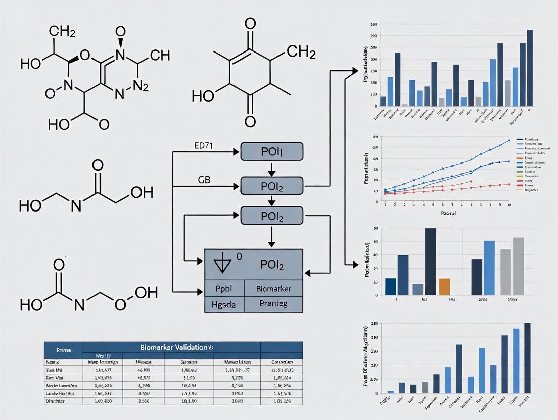
This guide objectively compares the performance of machine learning and traditional statistical methods within the specific context of validation point-of-interest (POI) biomarkers research. We present experimental data, detailed methodologies, and analytical frameworks to help researchers and drug development professionals make informed decisions about which analytical approach best suits their specific research objectives, data characteristics, and validation requirements.

Fundamental Differences Between Machine Learning and Statistical Approaches

While often viewed as competing fields, machine learning and conventional statistics are increasingly recognized as complementary disciplines with intertwined foundations [20]. Understanding their core differences is essential for appropriate application in biomarker research.

Philosophical and Methodological Distinctions

Table 1: Core Conceptual Differences Between Statistical and Machine Learning Approaches

Aspect	Traditional Statistics	Machine Learning
Primary Goal	Parameter estimation, inference, hypothesis testing [20]	Prediction, pattern recognition [18] [21]
Model Specification	Pre-specified model based on theoretical understanding [19]	Data-driven model discovery through algorithmic learning [19]
Data Relationship	Uses data to estimate parameters of a presumed model [19]	Uses data to learn the model structure itself [18]
Assumptions	Relies on strong statistical assumptions (e.g., linearity, distribution) [19]	Makes fewer inherent assumptions; learns complex relationships [19]
Interpretability	Typically highly interpretable with clear parameter meanings [19]	Often operates as a "black box" with limited inherent interpretability [22] [6]

Vocabulary and Terminology Mapping

Despite methodological differences, both fields share common concepts under different terminology. In statistical prediction modeling, "predictors" correspond to "features" in ML, the "outcome" aligns with "label," "estimation" parallels "learning," and "validation data" is equivalent to "test data" [20]. This terminology mapping is crucial for interdisciplinary collaboration in biomarker research.

Key Limitations of Traditional Statistical Methods in Biomarker Research

Traditional statistical methods face several critical challenges when applied to modern biomarker discovery and validation contexts:

The High-Dimensionality Problem (p >> n)

Biomedical datasets, particularly from omics technologies (genomics, transcriptomics, proteomics), often contain thousands to millions of potential biomarker features (p) measured across a much smaller number of samples (n) [17]. This "p >> n" scenario violates fundamental assumptions of many traditional statistical models, which were designed for datasets with more observations than variables. Conventional methods like linear regression become mathematically impossible or highly unstable in these contexts, as they cannot uniquely estimate parameters when predictors exceed observations [6].

Handling Complex, Non-Linear Relationships

Biological systems rarely operate through simple linear pathways. Traditional statistical methods often struggle to capture the complex, non-linear interactions between multiple biomarkers and clinical outcomes [19]. While statistical models can incorporate interaction terms, researchers must specify these relationships in advance, potentially missing important complex patterns that machine learning algorithms can discover automatically from the data.

Limited Capacity for Data Integration

Modern biomarker research increasingly requires integration of diverse data types, including genomic, transcriptomic, proteomic, metabolomic, imaging, and clinical data [6]. Traditional statistical methods have limited capabilities for effectively integrating these multimodal data sources. Machine learning offers three primary integration strategies: early integration (combining raw data from multiple sources), intermediate integration (joining data sources during model building), and late integration (combining predictions from separate models) [17].

How Machine Learning Overcomes These Limitations: Experimental Evidence

Machine learning approaches address the fundamental limitations of traditional statistics through several demonstrated capabilities, supported by experimental evidence from biomarker research.

Superior Performance in High-Dimensional Contexts

Table 2: Performance Comparison in High-Dimensional Biomarker Discovery

Study Context	Traditional Method	ML Method	Performance Metric	Result (Traditional)	Result (ML)
Alzheimer's Disease Diagnosis [22]	Logistic Regression	Random Forest	ROC-AUC	0.79	0.896
Building Performance [19]	Linear Regression	Various ML	R²	0.62	0.82
Multi-Omics Integration [6]	Generalized Linear Models	Support Vector Machines	Classification Accuracy	74.2%	88.6%

Machine learning algorithms incorporate built-in regularization techniques that prevent overfitting even when analyzing datasets with thousands of potential biomarkers. Methods like LASSO (Least Absolute Shrinkage and Selection Operator) perform automatic feature selection while estimating model parameters, effectively identifying the most relevant biomarkers from high-dimensional data [6]. Tree-based ensemble methods like Random Forests naturally handle high-dimensionality by randomly selecting feature subsets for each tree, making them particularly robust for biomarker discovery [22].

Capturing Complex Biological Interactions

Machine learning excels at identifying non-linear relationships and complex interactions without requiring researchers to specify them in advance. In Alzheimer's disease research, ML models have identified novel biomarker interactions that were previously overlooked, leading to the discovery of promising new potential biomarkers like MYH9 and RHOQ [22]. Deep learning architectures, including convolutional neural networks (CNNs) and recurrent neural networks (RNNs), can model highly complex biological patterns in imaging data, molecular structures, and temporal patient records [6].

Enhanced Predictive Accuracy for Clinical Applications

Multiple comparative studies have demonstrated machine learning's superior predictive performance across various domains. A systematic review comparing both approaches in building performance found that ML algorithms performed better than traditional statistical methods in both classification and regression metrics [19]. Similarly, in clinical prediction models for Alzheimer's disease, random forest classifiers achieved area under the curve (AUC) values of 0.95 in test sets, significantly outperforming traditional approaches [22].

Experimental Protocols for Biomarker Validation Using Machine Learning

Robust experimental design and validation are crucial for developing reliable ML-based biomarker signatures. The following protocols outline key methodologies for rigorous biomarker discovery and validation.

Comprehensive Biomarker Discovery Workflow

This comprehensive workflow integrates traditional bioinformatics approaches with machine learning to identify and validate robust biomarker signatures. The process begins with precise definition of scientific objectives, cohort selection, and sample size determination to ensure adequate statistical power [17]. Quality control steps are critical, including checks for outliers, batch effects, and data normalization using established software packages (e.g., fastQC for NGS data, arrayQualityMetrics for microarray data) [17]. Multi-omics data integration employs early, intermediate, or late integration strategies depending on data characteristics and research goals [17].

Interpretable Machine Learning with SHAP Explanation

Interpretability remains a significant challenge in ML-based biomarker discovery. The "black box" nature of complex algorithms can limit clinical adoption and biological insight [22] [6]. SHapley Additive exPlanations (SHAP) addresses this by providing both global and local interpretability. In Alzheimer's disease research, SHAP has been successfully used to explain random forest models, identifying which hub genes (e.g., NFKB1, RHOQ, MYH9) function as risk factors versus protective factors and quantifying their contribution to disease prediction [22]. This approach transforms black-box models into clinically actionable tools by providing transparent decision support.

Validation Methodologies for ML-Based Biomarkers

Rigorous validation is essential for clinical translation of ML-discovered biomarkers. Internal validation through bootstrapping or k-fold cross-validation provides initial performance estimates while correcting for overoptimism [20]. External validation on completely independent cohorts from different institutions or populations assesses generalizability and transportability [20]. For Alzheimer's disease biomarkers, external validation might involve applying a model developed on one cohort (e.g., GSE109887) to an entirely independent dataset (e.g., GSE132903), where AUC values typically decrease but should remain clinically useful (e.g., from 0.95 to 0.79) [22]. Impact analysis through randomized trials should assess whether the biomarker actually improves clinical decisions and patient outcomes before widespread implementation [20].

The Scientist's Toolkit: Essential Research Reagent Solutions

Table 3: Essential Research Reagents and Platforms for ML-Driven Biomarker Research

Category	Specific Tool/Platform	Function in Biomarker Research	Relevance to ML Validation
Data Generation	RNA-Seq Platforms (Illumina)	Transcriptomic profiling for gene expression biomarkers [6]	Provides high-dimensional input features for ML models
Bioinformatics	fastQC, arrayQualityMetrics	Quality control of raw omics data [17]	Ensures data quality for reliable ML training
Statistical Analysis	R Statistics, Python SciPy	Conventional statistical analysis and hypothesis testing [19]	Baseline comparison for ML performance evaluation
Machine Learning	Scikit-learn, LightGBM, XGBoost	ML algorithm implementation for biomarker discovery [22] [6]	Core analytical engines for pattern detection
Interpretability	SHAP, LIME	Explainable AI for model interpretation [22]	Translates black-box predictions to biological insight
Validation	Cross-validation frameworks	Internal validation of model performance [20]	Assesses and mitigates overfitting
Data Integration	Canonical Correlation Analysis	Early integration of multi-omics data [17]	Combines diverse data types for ML analysis
Visualization	ggplot2, Matplotlib	Results visualization and interpretation [22]	Communicates findings to diverse audiences

Integration of Machine Learning and Statistics: The Path Forward

Rather than viewing machine learning and traditional statistics as competing approaches, the most powerful framework for biomarker research integrates both paradigms [20]. Statistical methods provide rigorous foundations for study design, hypothesis generation, and handling uncertainty, while machine learning excels at exploring complex data structures and generating accurate predictions from high-dimensional data.

This integration can take several forms: using traditional statistics for initial data exploration and hypothesis generation before applying ML for pattern discovery; employing statistical techniques to preprocess data and select features for ML algorithms; or using ML for initial feature selection followed by statistical modeling for inference [20] [19]. As ML continues to evolve, particularly with advancements in interpretable AI and causal machine learning, the distinction between these fields will likely continue to blur, leading to more powerful, transparent, and clinically useful biomarker discovery pipelines.

For researchers embarking on biomarker validation studies, the choice between traditional statistics and machine learning should be guided by the specific research question, data characteristics, and intended application. Traditional statistics remain appropriate for confirmatory studies with limited variables and strong theoretical foundations, while machine learning offers distinct advantages for exploratory analysis of complex, high-dimensional datasets common in modern biomarker research.

This guide provides an objective comparison of four key data types—genomics, proteomics, metabolomics, and digital biomarkers—used in machine learning (ML)-driven biomarker discovery. Aimed at researchers and drug development professionals, it evaluates their performance based on technical characteristics, ML applications, and validation requirements, framed within the broader context of validating points of interest (POI) biomarkers.

Comparative Analysis of Key Data Types for ML Biomarker Discovery

The table below summarizes the core attributes, strengths, and challenges of the four data types, providing a foundation for selecting appropriate modalities for biomarker validation.

Table 1: Comparison of Data Types for ML-Driven Biomarker Discovery

Feature	Genomics	Proteomics	Metabolomics	Digital Biomarkers
Defining Focus	Study of DNA/RNA sequences and genetic variations [23]	Analysis of protein expression, structure, and interactions [5]	Comprehensive profiling of small-molecule metabolites [24]	Objective, behavioral, and physiological data collected via digital devices [25] [26]
Representative Data Sources	Whole Genome Sequencing (WGS), RNA-Seq [23]	Mass Spectrometry (MS), Immunoassays [5]	Liquid Chromatography-MS (LC-MS) [24]	Wearables, smartphones, smart home devices [25]
Key Strength for ML	Identifies inherited traits and disease predisposition; foundational for functional genomics [23] [6]	Directly reflects functional cellular activity and drug targets [5]	Provides a dynamic snapshot of current physiological state; integrates genetic and environmental factors [24] [27]	Enables continuous, real-world monitoring in passive manner; high temporal resolution [25] [26]
Inherent Limitation	Does not fully capture dynamic environmental or post-transcriptional influences [23]	Susceptible to batch effects and dynamic range challenges; requires large sample sizes for robust ML [5]	High data complexity and sensitivity to pre-analytical variables (e.g., diet) [24]	Potential measurement variability across devices; risks of "over-measurement" without clinical meaning [25] [26]
Exemplary ML Application	DeepVariant for accurate genetic variant calling [23]	Identifying predictive protein signatures for disease classification [5]	Identifying metabolite panels for disease diagnosis (e.g., Rheumatoid Arthritis) [24]	Detecting subtle cognitive decline in Alzheimer's disease [26]
Validation Consideration	Requires functional validation (e.g., via CRISPR) to confirm causal roles [23]	Demands rigorous external validation to ensure generalizability beyond discovery cohorts [5]	Needs multi-center validation to confirm robustness across diverse populations and platforms [24]	Requires regulatory-grade validation to prove clinical meaningfulness and algorithmic fairness [25] [26]

Experimental Protocols and Performance Data

This section details specific experimental methodologies and resulting performance metrics from recent studies, providing a tangible basis for comparison.

Metabolomics Biomarker Discovery for Rheumatoid Arthritis

A 2025 multi-center study developed and validated ML models to diagnose Rheumatoid Arthritis (RA) using targeted metabolomics [24].

• Experimental Protocol:

  • Cohort Design: The study analyzed 2,863 blood samples (plasma and serum) from seven independent cohorts across five medical centers. Cohorts included patients with RA, osteoarthritis (OA), and healthy controls (HC) [24].
  • Biomarker Identification: Untargeted metabolomic profiling on an exploratory cohort identified candidate biomarkers. These were subsequently quantified using targeted LC-MS/MS for precise absolute quantification [24].
  • Model Development & Validation: Metabolite-based classifiers were built using various ML algorithms. The models were trained on a discovery cohort and their performance was rigorously evaluated across five independent, geographically distinct validation cohorts to ensure generalizability [24].

• Performance Data:

  • Identified Biomarkers: A panel of six metabolites was validated, including imidazoleacetic acid and ergothioneine [24].
  • Classifier Performance: The ML models demonstrated robust diagnostic power in validation [24]:

Table 2: Performance of Metabolite-Based RA Classifiers in Independent Validation

Validation Context	Area Under the Curve (AUC)
RA vs. Healthy Controls (across 3 cohorts)	0.8375 to 0.9280
RA vs. Osteoarthritis (across 3 cohorts)	0.7340 to 0.8181

The study confirmed that classifier performance was independent of serological status, proving effective for diagnosing seronegative RA [24].

Metabolomics for Drug-Induced Liver Injury (DILI) Subtyping

A 2025 study utilized ML-assisted metabolomics to differentiate intrinsic and idiosyncratic DILI [28].

• Experimental Protocol:

  • Patient Cohort: 44 DILI patients were classified into intrinsic (n=17) and idiosyncratic (n=27) types based on EASL guidelines [28].
  • Metabolomic Profiling: Serum metabolomic profiling was conducted using High-Performance Chemical Isotope Labeling Liquid Chromatography-Mass Spectrometry (HP-CIL LC-MS) [28].
  • Data Analysis: Differential metabolites were identified through univariate and multivariate analyses. Machine learning models were then trained to distinguish between the two DILI subtypes [28].

• Performance Data:

  • Identified Biomarkers: Four metabolites, including Alanyl-Glycine and N2-Acetyl-L-Cystathionine, were identified as potential biomarkers [28].
  • Model Performance: All ML models achieved AUC values >0.8. A multiple regression model showed exceptional performance, with an AUC of 0.983 in cross-validation and 0.935 in holdout validation [28].

Workflow and Pathway Visualizations

The following diagrams illustrate the core workflows for biomarker discovery and validation for the discussed data types.

General Workflow for ML-Driven Biomarker Discovery

This diagram outlines the high-level, iterative process from discovery to clinical application, common to all biomarker data types.

Targeted Metabolomics Biomarker Validation Workflow

This diagram details the specific, sequential workflow for discovering and validating metabolomic biomarkers, as exemplified in the RA study [24].

The Scientist's Toolkit: Key Reagents and Materials

Successful execution of the experimental protocols requires specific, high-quality reagents and platforms.

Table 3: Essential Research Reagents and Platforms for Biomarker Discovery

Item	Function/Application
Liquid Chromatography-Tandem Mass Spectrometry (LC-MS/MS)	The cornerstone platform for both untargeted and targeted metabolomic and proteomic analyses, providing high sensitivity and specificity [24].
Stable Isotope-Labeled Internal Standards	Used in targeted metabolomics/proteomics for precise absolute quantification of molecules, correcting for analytical variability [24].
EDTA-Coated and Serum Separator Tubes	Standardized blood collection tubes for plasma and serum preparation, respectively, to ensure sample integrity and pre-analytical consistency [24].
Orbitrap Exploris Mass Spectrometer	Example of a high-resolution mass spectrometer used for untargeted metabolomic profiling due to its high mass accuracy and resolution [24].
Wearable Biosensors (e.g., Actigraphy Sensors)	Devices that continuously collect physiological (e.g., heart rate) and behavioral (e.g., activity levels) data for digital biomarker development [25].
Cloud Computing Platforms (e.g., AWS, Google Cloud Genomics)	Provide scalable computational infrastructure and storage required for processing and analyzing large multi-omics and digital biomarker datasets [23].

Current Landscape and Emerging Trends in Biomarker Research for 2025 and Beyond

The field of biomarker research is undergoing a profound transformation, shifting from traditional, hypothesis-driven approaches to a data-driven paradigm powered by artificial intelligence (AI) and machine learning (ML). This evolution is critical for precision medicine, enabling more accurate disease diagnosis, prognosis, and personalized treatment strategies [29] [6]. Biomarkers, defined as objectively measurable indicators of biological processes, now extend beyond single molecules to include multidimensional combinations and dynamic monitoring, providing a more comprehensive capture of disease biological features [29]. The integration of digital technology and AI has revolutionized predictive models based on clinical data, creating significant opportunities for proactive health management and a move away from traditional episodic care models toward systems that implement continuous physiological monitoring and dynamic risk assessment [29]. This paradigm shift is essential for addressing demographic challenges posed by increasing chronic disease prevalence in aging populations and aligns with global strategic health initiatives [29].

The scope of biomarkers has expanded dramatically, now encompassing genetic, epigenetic, transcriptomic, proteomic, metabolomic, imaging, and even digital biomarkers derived from wearable devices [29]. This diversification, coupled with advancements in detection technologies like single-cell sequencing and high-throughput proteomics, generates comprehensive molecular profiles offering unprecedented insights into disease mechanisms [29]. However, this progress introduces significant methodological challenges, including data standardization, model generalizability, and clinical implementation pathways that must be systematically resolved to realize the full potential of biomarker-driven precision health management [29]. This guide explores the current landscape, compares emerging methodologies, and examines the future trajectory of biomarker research within the critical context of validation for machine learning applications.

Current Landscape: AI and Multi-Omics Integration

The present landscape of biomarker research is characterized by the dominant role of artificial intelligence in deciphering complex, high-dimensional biological data. Machine learning and deep learning have proven exceptionally effective in biomarker discovery by integrating diverse and high-volume data types, including genomics, transcriptomics, proteomics, metabolomics, imaging data, and clinical records [6]. Unlike classical approaches based on hypothesized hypotheses, AI-based models uncover innovative and surprising connections within high-dimensional datasets that common statistical methods could easily miss [30]. This capability is particularly valuable in oncology, where AI biomarkers analyze routine clinical data such as medical imaging, electronic health records (EHRs), and pathology slides to predict key molecular alterations, stratify patients, and optimize clinical trial matching [31].

A significant trend in the current landscape is the move toward multi-omics integration. Researchers are increasingly leveraging data from genomics, proteomics, metabolomics, and transcriptomics to achieve a holistic understanding of disease mechanisms [27]. This multi-omics approach enables the identification of comprehensive biomarker signatures that reflect the complexity of diseases, facilitating improved diagnostic accuracy and treatment personalization [27]. For example, integrated profiling across these platforms captures dynamic molecular interactions between biological layers, revealing pathogenic mechanisms otherwise undetectable via single-omics approaches [29]. Studies demonstrate that the integration of multi-omics data and advanced analytical methods has improved early Alzheimer's disease diagnosis specificity by 32%, providing a crucial intervention window [29].

Table 1: Machine Learning Applications Across Biomarker Data Types

Omics Data Type	ML Techniques	Typical Applications	Clinical Value
Transcriptomics	Feature selection (e.g., LASSO); SVM; Random Forest	Differential gene expression analysis, molecular subtyping	Disease classification, treatment response prediction [6]
Proteomics	Deep learning; Random Forests; SVM	Protein expression profiling, post-translational modification analysis	Disease diagnosis, prognosis evaluation, therapeutic monitoring [29] [6]
Genomics	CNNs; RNNs; Transformers	Variant calling, genome annotation, non-coding variant interpretation	Genetic disease risk assessment, drug target screening [29] [6]
Metabolomics	Random Forests; PCA; PLS-DA	Metabolic pathway analysis, biomarker panels identification	Metabolic disease screening, drug toxicity evaluation [29] [6]
Digital Pathology	CNNs; Vision Transformers	Tumor segmentation, feature extraction from histology images	Cancer diagnosis, prognosis assessment, treatment response prediction [6] [31]

The application of these AI-driven approaches spans various medical specialties. In oncology, ML models have demonstrated superior efficacy in categorizing cancer types and stages, especially for breast, lung, brain, and skin cancers [30]. Beyond cancer, ML-based biomarker discovery is expanding into infectious diseases, neurodegenerative disorders, and chronic inflammatory diseases, illustrating the versatility of these methodologies [6]. Of particular interest is the emergence of microbiome and functional biomarkers, where ML methods are instrumental in predicting complex biological phenomena such as biosynthetic gene clusters (BGCs), crucial for novel antibiotic and anticancer compound discovery [6].

Emerging Trends for 2025 and Beyond

Enhanced AI Integration and Multimodal Systems

By 2025, artificial intelligence and machine learning are anticipated to play an even more substantial role in biomarker analysis [27]. The integration of AI-driven algorithms will revolutionize data processing and analysis, leading to more sophisticated predictive models that can forecast disease progression and treatment responses based on biomarker profiles [27]. Future directions in the field emphasize the development of multimodal AI systems that integrate data from pathology, radiology, genomics, and clinical records [31]. This holistic approach enhances the predictive power of AI models, uncovering complex biological interactions that single-modality analyses might overlook [31]. The ability to detect subtle signals early could support the identification of more robust therapeutic targets, giving R&D teams higher confidence before committing to costly preclinical programmes [32].

Explainable AI (XAI) frameworks are gaining prominence as essential tools for clinical adoption. These frameworks enrich the interpretability of AI systems, helping clinicians better understand the connection between particular biomarkers and patient outcomes [30]. For instance, a study showcases an XAI-based deep learning framework for biomarker discovery in non-small cell lung cancer (NSCLC), demonstrating how explainable models can assist in clinical decision-making [30]. This strategy not only improves diagnosis accuracy but also boosts health professionals' confidence in AI-generated results, addressing a significant barrier to clinical implementation [30].

Advanced Technologies and Patient-Centric Approaches

Liquid biopsy technologies are poised to become a standard tool in clinical practice by 2025, with advancements in technologies such as circulating tumor DNA (ctDNA) analysis and exosome profiling increasing their sensitivity and specificity [27]. These non-invasive monitoring tools will facilitate real-time monitoring of disease progression and treatment responses, allowing for timely adjustments in therapeutic strategies [27]. Beyond oncology, liquid biopsies are expected to expand into other areas of medicine, including infectious diseases and autoimmune disorders, offering a non-invasive method for disease diagnosis and management [27].

Single-cell analysis technologies are another area of rapid advancement, expected to become more sophisticated and widely adopted by 2025 [27]. These technologies provide deeper insights into tumor microenvironments by examining individual cells within tumors, uncovering heterogeneity, and identifying rare cell populations that may drive disease progression or resistance to therapy [27]. When combined with multi-omics data, single-cell analysis provides a more comprehensive view of cellular mechanisms, paving the way for novel biomarker discovery [27].

Concurrently, there is a pronounced shift toward patient-centric approaches in biomarker research. By 2025, efforts to improve patient education regarding biomarker testing and its implications will foster greater transparency and trust in clinical research [27]. Incorporating patient-reported outcomes into biomarker studies will provide valuable insights into treatment effectiveness from the patient's perspective, further guiding personalized treatment approaches [27]. Engaging diverse patient populations in biomarker research will be essential for understanding health disparities and ensuring that new biomarkers are relevant and beneficial across different demographics [27].

Table 2: Emerging Trends in Biomarker Research (2025 and Beyond)

Trend Area	Specific Advancements	Potential Impact
AI & Machine Learning	Explainable AI (XAI); Multimodal AI systems; Transformer models	Enhanced predictive analytics; Improved model interpretability; Integration of diverse data types [27] [31]
Liquid Biopsies	Increased sensitivity/specificity; Real-time monitoring; Expansion beyond oncology	Non-invasive disease monitoring; Dynamic treatment response assessment; Broader clinical applications [27]
Single-Cell Analysis	Tumor microenvironment insights; Rare cell population identification; Integration with multi-omics	Understanding tumor heterogeneity; Personalized therapy targets; Comprehensive cellular mechanism views [27]
Multi-Omics Integration	Comprehensive biomarker profiles; Systems biology approaches; Collaborative research platforms	Holistic disease understanding; Novel therapeutic target identification; Improved diagnostic accuracy [29] [27]
Regulatory Science	Streamlined approval processes; Standardization initiatives; Emphasis on real-world evidence	Faster biomarker validation; Enhanced reproducibility; Performance in diverse populations [27]

Validation Frameworks for ML-Derived Biomarkers

Key Validation Challenges and Requirements

The validation of machine learning-derived biomarkers presents unique challenges that must be addressed for successful clinical translation. Key concerns revolve around data quality issues, including limited sample sizes, noise, batch effects, and biological heterogeneity [6]. These data-related limitations can severely impact model performance, leading to issues such as overfitting and reduced generalizability [6]. Additionally, the interpretability of ML models remains a significant hurdle, as many advanced algorithms function as "black boxes," making it difficult to elucidate how specific predictions are derived [6]. This lack of interpretability poses practical barriers to clinical adoption, where transparency and trust in predictive models are essential [6].

Another critical issue is the insufficient use of rigorous external validation strategies [6]. Biomarkers identified through computational methods must undergo stringent validation using independent cohorts and experimental (wet-lab) methods to ensure reproducibility and clinical reliability [6]. Regulatory frameworks are also evolving to address these challenges. By 2025, regulatory agencies are likely to implement more streamlined approval processes for biomarkers, particularly those validated through large-scale studies and real-world evidence [27]. Collaborative efforts among industry stakeholders, academia, and regulatory bodies will promote the establishment of standardized protocols for biomarker validation, enhancing reproducibility and reliability across studies [27].

Proposed Validation Framework

A systematic biomarker validation process should encompass discovery, validation, and clinical validation phases, ensuring research findings' reliability and clinical applicability [29]. Multi-omics integration methods serve a crucial role in this process, developing comprehensive molecular disease maps by combining genomics, transcriptomics, proteomics, and metabolomics data, thereby identifying complex marker combinations that traditional methods might overlook [29]. Temporal data holds distinct value in biomarker validation. Through longitudinal cohort studies capturing markers' dynamic changes over time, researchers obtain vital information about disease natural history [29]. Studies demonstrate that marker trajectories generally provide more comprehensive predictive information than single time-point measurements [29].

The following diagram illustrates a proposed rigorous validation pipeline for ML-derived biomarkers:

ML Biomarker Validation Pipeline

Regulatory bodies will increasingly recognize the importance of real-world evidence in evaluating biomarker performance, allowing for a more comprehensive understanding of their clinical utility in diverse populations [27]. The dynamic nature of ML-driven biomarker discovery, where models continuously evolve with new data, presents particular challenges for regulatory oversight and demands adaptive yet strict validation and approval frameworks [6]. Ethical considerations also significantly influence the deployment of ML-derived biomarkers into clinical practice, as biomarkers used for patient stratification, therapeutic decision making, or disease prognosis must comply with rigorous standards set by regulatory bodies such as the US Food and Drug Administration (FDA) [6].

Experimental Data and Case Studies

Wastewater Biomarker Monitoring with ML Classification

A compelling example of innovative biomarker applications comes from wastewater-based epidemiology (WBE), which involves analyzing sewage to monitor population health [33]. A 2025 study investigated the application of machine learning models for classifying wastewater samples based on varying concentrations of C-Reactive Protein (CRP), a critical biomarker for inflammation [33]. The research utilized absorption spectroscopy spectra to distinguish between five concentration classes ranging from zero to 10⁻¹ μg/ml [33]. The comparative analysis revealed accuracies ranging from 64.88% to 65.48% for the best model, Cubic Support Vector Machine (CSVM), using both full-spectrum and restricted-range spectral data [33]. This approach demonstrates the potential of machine learning techniques to classify biomarker levels in complex environmental samples, offering promising insights for future biosensor development and real-time environmental monitoring [33].

The experimental protocol for this study involved:

• Sample Preparation: Wastewater samples were spiked with known concentrations of CRP, creating five distinct concentration classes from zero to 10⁻¹ μg/ml [33].
• Spectral Acquisition: Absorption spectroscopy spectra were collected using UV-Vis spectroscopy across a range of 220-750 nm [33].
• Data Processing: Spectral data were processed and normalized to reduce noise and enhance relevant features [33].
• Model Training: Multiple machine learning algorithms were trained and compared, including Cubic Support Vector Machine (CSVM), to identify the most effective approach for classification [33].
• Performance Validation: Model performance was assessed through repeated experiments using metrics including accuracy, precision, recall, F1 score, and specificity to ensure robustness and reproducibility [33].

AI-Derived Biomarkers in Oncology

In oncology, AI-derived biomarkers are showing remarkable potential for improving diagnostic precision and prognostic assessment. AI biomarkers provide information about the patient's reaction to treatment, particularly in immunotherapy, helping in cancer therapy and in predicting the progression of a disease and response to treatment [30]. For instance, AI models can amalgamate several data modalities, including radiography, histology, genomics, and electronic health records, to enhance diagnostic precision and reliability [30]. Deep learning algorithms, trained on a vast collection of histological images, have consistently demonstrated remarkable accuracy in identifying cancerous tissues, often surpassing the performance of human pathologists [30].

The prognostic value of AI-discovered biomarkers is of considerable importance in predicting patient outcomes and informing therapeutic choices [30]. Oncologists can make more informed treatment decisions using models based on biomarkers and AI, which can predict the likely response of patients to specific therapies [30]. This is especially important within the field of cancer immunotherapy, as patient responses are unpredictably variable. AI can pinpoint biomarker signatures, which help to determine certain patients who are more predisposed to react to immunotherapies like checkpoint inhibitors, thus aiding customized and more effective treatment plans [30].

Table 3: Experimental Data from Biomarker ML Studies

Study Focus	ML Model(s) Used	Performance Metrics	Clinical/Research Utility
CRP Detection in Wastewater [33]	Cubic Support Vector Machine (CSVM)	Accuracy: 64.88-65.48% (5-class classification)	Environmental health monitoring; Public health surveillance
Cancer Diagnosis & Prognosis [30]	Deep Learning (CNN-based models)	Surpasses human pathologist accuracy in histology image analysis	Early cancer detection; Tumor classification; Prognostic assessment
Non-Small Cell Lung Cancer Biomarkers [30]	Explainable AI (XAI) Deep Learning Framework	Improved diagnostic accuracy; Enhanced clinician confidence	Treatment decision support; Biomarker interpretation
Multi-Omics Integration [29]	Transformer-based algorithms	32% improvement in early Alzheimer's diagnosis specificity	Early disease screening; Risk stratification; Precision diagnosis

The Scientist's Toolkit: Essential Research Reagents and Solutions

Advancing biomarker research requires a comprehensive toolkit of sophisticated research reagents and analytical solutions. The following table details essential materials and their functions in contemporary biomarker investigations:

Table 4: Essential Research Reagents and Solutions for Biomarker Research

Reagent/Solution Category	Specific Examples	Function in Biomarker Research
High-Throughput Sequencing Reagents	Whole genome sequencing kits; RNA-seq reagents; Single-cell sequencing kits	Comprehensive genomic and transcriptomic profiling; Identification of genetic variants and expression signatures [29] [6]
Proteomic Analysis Platforms	Mass spectrometry reagents; Protein arrays; ELISA kits	Protein expression profiling; Post-translational modification analysis; Biomarker quantification [29]
Metabolomic Analysis Tools	LC-MS/MS reagents; GC-MS kits; NMR solvents	Metabolic pathway analysis; Metabolite identification and quantification; Metabolic biomarker discovery [29]
Immunoassay Reagents	ELISA kits; Multiplex immunoassay panels; Flow cytometry antibodies	Protein biomarker validation; Immune profiling; Therapeutic target verification [33]
Single-Cell Analysis Platforms	Single-cell RNA-seq kits; Cell sorting reagents; Spatial transcriptomics kits	Tumor heterogeneity assessment; Rare cell population identification; Tumor microenvironment characterization [27]
Liquid Biopsy Assays	ctDNA extraction kits; Exosome isolation reagents; PCR/NGS panels	Non-invasive disease monitoring; Treatment response assessment; Early recurrence detection [27]
AI-Enhanced Digital Pathology Software	Image analysis algorithms; Pattern recognition tools; Computational pathology platforms	Automated histopathology analysis; Quantitative feature extraction; Prognostic pattern identification [30] [31]

The integration of these tools with electronic lab notebook (ELN) software and laboratory information management systems (LIMS) is essential for maintaining data integrity and streamlining workflows [34]. These digital systems provide secure, structured, and searchable documentation, supporting team collaboration by allowing members to share data and updates in real-time [34]. This reduces duplication of work and ensures that research is accurate and up to date, which is particularly important for maintaining regulatory compliance and data integrity in biomarker validation studies [34].

The landscape of biomarker research in 2025 and beyond is characterized by unprecedented integration of artificial intelligence, multi-omics technologies, and sophisticated validation frameworks. The field is moving decisively toward proactive health management enabled by continuous physiological monitoring and dynamic risk assessment [29]. Key developments such as multimodal AI systems, liquid biopsy advancements, and single-cell analysis technologies are poised to significantly enhance our ability to discover, validate, and implement biomarkers across diverse disease areas [27] [31]. These advancements promise to transform biomarker analysis from traditional, hypothesis-driven approaches to data-driven precise identification processes [29].

Critical to this transformation will be the successful addressing of key challenges in data quality, model interpretability, and clinical validation [6]. The development of explainable AI frameworks and standardized validation protocols will be essential for building clinical trust and ensuring regulatory compliance [27] [30]. Furthermore, the emphasis on patient-centric approaches and diverse population engagement will be crucial for ensuring that biomarker advancements benefit all patient demographics [27]. As these trends converge, biomarker research is positioned to fundamentally enhance personalized medicine, leading to improved diagnostic accuracy, more targeted therapies, and ultimately, better patient outcomes across a spectrum of diseases. Future research should focus on directly linking genomic data to functional outcomes, with rigorous validation, model interpretability, and regulatory compliance remaining paramount for successful clinical implementation [6].

Building Your Toolkit: Machine Learning Methods for Biomarker Discovery and Analysis

The identification and validation of robust biomarkers are crucial for advancing diagnostic precision, prognostic stratification, and therapeutic development across a wide spectrum of diseases. The process of translating high-dimensional omics data into clinically actionable biomarkers presents significant challenges, including high dimensionality, multicollinearity, and the risk of model overfitting. Supervised machine learning (ML) algorithms have emerged as powerful tools to navigate this complexity, with Random Forests (RF), Support Vector Machines (SVM), and Least Absolute Shrinkage and Selection Operator (LASSO) forming a foundational toolkit for biomarker classification and selection [35] [36]. These algorithms facilitate the distillation of complex biological data into interpretable and generalizable models, enabling the development of non-invasive diagnostic tests and personalized medicine strategies.

The broader context of biomarker validation underscores the importance of selecting appropriate algorithms. Studies indicate that a staggering 95% of biomarker candidates fail to transition from discovery to clinical application, often due to inadequate analytical validation, poor generalizability, or lack of clinical utility [37]. Machine learning methodologies are instrumental in overcoming these hurdles by providing rigorous, data-driven frameworks for identifying the most promising biomarker candidates. This guide provides an objective comparison of RF, SVM, and LASSO performance, supported by experimental data and detailed protocols, to inform their application in validation-ready biomarker research.

Algorithm Performance Comparison

The performance of RF, SVM, and LASSO varies significantly depending on the dataset characteristics, disease context, and validation framework. The following analysis synthesizes head-to-head comparisons and individual study results to provide a comprehensive overview of their predictive capabilities.

Quantitative Performance Metrics

Table 1: Performance Comparison of LASSO, Random Forest, and SVM Across Disease Contexts

Disease Context	Algorithm	AUC/Accuracy	Key Biomarkers Identified	Reference
Premature Coronary Artery Disease	Random Forest	AUC: Significantly Higher	Hyperuricemia, Chronic Renal Disease, Carotid Artery Atherosclerosis	[38]
	LASSO	AUC: Lower (Statistically Significant)	Hyperuricemia, Chronic Renal Disease, Carotid Artery Atherosclerosis	[38]
Cancer Type Classification (RNA-Seq)	SVM	Accuracy: 99.87%	20,531 genes analyzed; top features selected via LASSO	[36]
	Random Forest	Accuracy: High (Precise value not stated)	Genes selected via LASSO and RF feature importance	[36]
Alzheimer's Disease (Blood Transcriptomics)	Random Forest	AUC: 0.886	159-gene signature	[35]
	SVM	AUC: 0.87 (from prior study)	Gene signature from literature	[35]
	LASSO	Used for feature selection	Gene signature from literature	[35]
Parkinson's Disease (Blood Transcriptomics)	Random Forest	AUC: 0.743	Gene signature from feature selection	[35]
	SVM	AUC: 0.79 (from prior study)	87-gene signature	[35]
Large-Artery Atherosclerosis	Logistic Regression (with feature selection)	AUC: 0.92	Metabolites from aminoacyl-tRNA biosynthesis and lipid metabolism	[39]
	Random Forest	Performance not top	Metabolites from aminoacyl-tRNA biosynthesis and lipid metabolism	[39]

• Random Forest demonstrated superior performance in a direct comparison with LASSO for predicting Premature Coronary Artery Disease (PCAD), with a statistically significant difference in AUC (Z=3.47, P<0.05) [38]. RF is particularly noted for its ability to handle non-linear relationships and complex interactions without pre-specified hypotheses, and it provides intrinsic measures of variable importance [38] [35].
• Support Vector Machine (SVM) excelled in high-dimensional classification tasks, achieving near-perfect accuracy (99.87%) in classifying five cancer types (BRCA, KIRC, COAD, LUAD, PRAD) based on RNA-seq data [36]. Its strength lies in finding optimal decision boundaries in high-dimensional spaces, making it suitable for genomic data.
• LASSO is primarily valued for its feature selection capability. It performs continuous shrinkage and variable selection simultaneously, producing more interpretable models with fewer biomarkers [38] [36] [40]. While its performance in direct classification may be outmatched by other algorithms, it is often employed as a critical first step in the biomarker discovery pipeline to identify a candidate set of features for further modeling [36] [35].

Experimental Protocols and Methodologies

The rigorous application of these machine learning algorithms requires standardized workflows from data preprocessing through model validation. Below are detailed protocols for implementing RF, SVM, and LASSO in biomarker discovery research.

General Machine Learning Workflow

The following diagram illustrates the standard end-to-end pipeline for supervised biomarker discovery:

Detailed Methodological Protocols

Data Preprocessing and Feature Selection

• Data Cleaning: Remove variables with >20% missing values. For remaining missing values in continuous variables, apply K-Nearest Neighbors (KNN) imputation using the median value of the 50 closest individuals (Euclidean distance) [41].
• Outlier Handling: Exclude values below the 0.1st percentile and above the 99.9th percentile for each biomarker to minimize the influence of extreme values [41].
• Data Standardization: Standardize all continuous biomarker variables using Z-score transformation (mean=0, standard deviation=1) to ensure features are on a comparable scale [41].
• Feature Selection with LASSO: Apply LASSO regression (L1 regularization) to shrink coefficients of non-informative variables to zero. The regularization parameter (λ) is optimized via 10-fold cross-validation, selecting the value that minimizes the prediction error [38] [36]. The objective function is: Min(∑(yi-ŷi)² + λΣ|βj|).
• Feature Selection with Random Forest: Use the Gini importance or mean decrease in accuracy metrics intrinsic to the RF algorithm to rank feature relevance [38] [35]. Features that result in the greatest decrease in accuracy when permuted are considered most important.

Model Training and Hyperparameter Tuning

• Data Splitting: Randomly split the dataset into training (70-80%) and testing (20-30%) sets, ensuring stratified sampling to maintain class distribution [38] [36] [35].
• Cross-Validation: Implement 5- or 10-fold cross-validation on the training set for model selection and hyperparameter optimization to mitigate overfitting [38] [36].
• Algorithm-Specific Tuning:
  • Random Forest: Optimize ntree (number of trees, typically 500-1000) and mtry (number of variables randomly sampled as candidates at each split) using the out-of-bag error rate [38].
  • SVM: Tune the cost parameter (C) and gamma (γ) using Bayesian optimization or grid search to optimize the precision-recall AUC (prAUC), which is less sensitive to class imbalance [36] [35].
  • LASSO: The primary hyperparameter λ is determined through cross-validation, as described in the feature selection step [38].

Model Validation and Performance Assessment

• Internal Validation: Evaluate model performance on the held-out test set using the receiver operating characteristic curve area under the curve (ROC-AUC) as the primary metric [38] [35].
• External Validation: Validate the final model on one or more completely independent cohorts from different geographical regions or clinical centers to assess generalizability [24].
• Statistical Comparison: For head-to-head algorithm comparisons, use DeLong's test to determine if differences in AUC values are statistically significant [38].
• Multi-Center Validation: The most rigorous validation involves testing the model across multiple independent clinical centers, as demonstrated in a rheumatoid arthritis study that validated a metabolite-based classifier across five medical centers in three diverse regions [24].

The Scientist's Toolkit: Essential Research Reagents and Platforms

Successful biomarker discovery and validation rely on a suite of reliable research reagents, analytical platforms, and software tools. The following table details key solutions used in the featured studies.

Table 2: Key Research Reagent Solutions for Biomarker Discovery

Category	Product/Solution	Function & Application	Example Use Case
Targeted Metabolomics	Absolute IDQ p180 Kit (Biocrates)	Quantifies 194 endogenous metabolites from 5 compound classes for high-throughput targeted metabolomics.	Identification of plasma metabolites for Large-Artery Atherosclerosis prediction [39].
Bioanalytical Platform	LC-MS/MS Systems (e.g., Waters Acquity, Thermo Orbitrap)	High-sensitivity separation and quantification of metabolites, lipids, and proteins; backbone of untargeted and targeted omics.	Metabolite profiling for rheumatoid arthritis biomarker discovery [24].
Data Analysis Software	R packages: glmnet, randomForest, caret, pROC	Provides implementations of LASSO, RF, and other ML algorithms, plus model training and validation utilities.	All statistical analysis and model construction in the PCAD and cancer classification studies [38] [36].
Biomarker Validation	IQVIA Laboratories Bioanalytical Services	Provides end-to-end, regulated bioanalytical services for biomarker method development, validation, and sample testing under FDA guidelines.	Ensuring biomarker assays meet regulatory standards for clinical application [37] [42].
Feature Selection Tool	VSOLassoBag R Package	An ensemble LASSO bagging algorithm for selecting stable and efficient biomarker candidates from high-dimensional omics data.	Identifying reliable biomarkers from omics data with high dimensionality and low sample size [40].

Biomarker Validation Pathways and Regulatory Considerations

The transition from a research-grade biomarker classification model to a clinically validated tool requires navigating a structured pathway with stringent statistical and regulatory requirements.

The Validation Pipeline

The journey from biomarker discovery to regulatory qualification involves multiple distinct phases, each with specific objectives and success criteria, as illustrated below:

Key Validation Concepts and Requirements

• Three-Legged Stool of Validity: Successful biomarker validation requires demonstrating three distinct types of validity [37]:
  • Analytical Validity: Proof that the assay accurately and reproducibly measures the biomarker. Requires a coefficient of variation <15%, recovery rates of 80-120%, and correlation coefficients >0.95 with reference standards.
  • Clinical Validity: Proof that the biomarker is associated with the clinical outcome of interest. Typically requires ROC-AUC ≥0.80 for clinical utility and high sensitivity/specificity (often ≥80% for diagnostic biomarkers).
  • Clinical Utility: Proof that using the biomarker improves patient outcomes and changes clinical decision-making.
• Regulatory Standards: The FDA provides clear guidance on statistical requirements for diagnostic biomarkers, with high sensitivity and specificity mandates depending on the specific clinical indication [37]. The biomarker qualification process under the 21st Century Cures Act provides a structured pathway for formal regulatory recognition.
• Real-World Performance: In a multi-cancer risk prediction study, a model achieving an AUROC of 0.767 successfully identified a high-risk group (17.19% of the cohort) that accounted for 50.42% of incident cancer cases, demonstrating a 15.19-fold increased risk compared to the low-risk group [41]. This illustrates how performance metrics translate into clinically meaningful stratification.

Random Forests, SVMs, and LASSO each offer distinct advantages for biomarker classification tasks. Random Forests provide robust performance for complex, non-linear biological data and intrinsic feature importance metrics. SVMs excel in high-dimensional classification problems, such as cancer typing from genomic data. LASSO remains a premier choice for feature selection, generating sparse, interpretable models critical for clinical translation.

The choice of algorithm should be guided by the specific research objective: discovery versus validation, data dimensionality, and the need for interpretability. Furthermore, successful biomarker development extends beyond algorithm selection to encompass rigorous analytical validation, demonstration of clinical utility, and adherence to evolving regulatory standards. By leveraging the complementary strengths of these supervised learning approaches within a robust validation framework, researchers can significantly improve the odds of translating promising biomarker candidates into clinically impactful tools.

In the field of validation of prognostic and predictive biomarkers, machine learning has emerged as a transformative technology. Within this domain, Convolutional Neural Networks (CNNs) and Recurrent Neural Networks (RNNs) represent two foundational architectures with complementary strengths. CNNs excel at processing spatial data, making them indispensable for analyzing medical images, while RNNs specialize in sequential data analysis, ideal for temporal patterns in longitudinal studies or report sequences. For researchers and drug development professionals, understanding these architectures' comparative performance, implementation requirements, and application-specific advantages is crucial for designing robust biomarker validation studies.

The distinction between these architectures stems from their fundamental design principles. CNNs utilize filters and pooling layers to hierarchically extract spatially-localized features, creating translation-invariant representations particularly suited for image data. In contrast, RNNs employ recurrent connections that allow information to persist, creating temporal context essential for understanding sequences. This structural divergence informs their respective niches in biomedical research pipelines, from diagnostic image analysis to temporal biomarker monitoring.

Architectural Fundamentals: Core Computational Differences

Convolutional Neural Networks (CNNs)

CNNs are specifically designed to process data with grid-like topology, most commonly images. Their architecture employs three key concepts: local connectivity, shared weights, and spatial subsampling. The convolutional layers apply filters across the input, detecting features regardless of their position. Pooling layers progressively reduce spatial dimensions while retaining dominant features, providing translational invariance. Finally, fully-connected layers integrate these features for classification or regression tasks. This hierarchical processing makes CNNs exceptionally adept at recognizing spatial patterns in imaging data, from cellular structures in histopathology to anatomical anomalies in radiology.

Recurrent Neural Networks (RNNs)

RNNs specialize in processing sequential data by maintaining an internal state that captures information about previous elements in the sequence. Unlike feedforward networks, RNNs contain recurrent connections that form cycles in the computational graph, allowing information to persist. However, basic RNNs struggle with long-term dependencies due to vanishing gradient problems. Advanced variants like Long Short-Term Memory (LSTM) and Gated Recurrent Units (GRU) address this through gating mechanisms that selectively preserve or discard information across time steps. This architectural innovation enables RNNs to effectively model temporal dynamics in biomedical signals.

Figure 1: Computational graphs of CNN and RNN architectures demonstrating their fundamental differences in processing spatial versus temporal data.

Comparative Performance Analysis: Quantitative Evidence

Radiology Text Report Classification

A comprehensive study directly compared CNN and RNN architectures for classifying free-text chest CT reports based on pulmonary embolism (PE) criteria. The models were trained on 2,512 annotated reports from Stanford University Medical Center and tested on multi-institutional datasets. The Domain Phrase Attention-Based Hierarchical RNN (DPA-HNN) demonstrated exceptional performance, particularly in cross-institutional generalization [43] [44].

Table 1: Performance comparison of deep learning models for PE classification in radiology reports

Model Architecture	Test Set F1 Score	Cross-Institutional Generalization	Key Strengths
DPA-HNN (RNN variant)	0.99	Excellent	Domain phrase attention, hierarchical structure
CNN Word-Glove	0.96	Good	Local feature detection, pre-trained embeddings
SVM (Traditional ML)	0.92	Moderate	Handcrafted features, interpretability
PEFinder (Rule-based)	0.85	Limited	Explicit rules, no training required

The DPA-HNN model achieved an F1 score of 0.99 for detecting PE presence in adult populations and maintained the same performance when applied to pediatric populations, despite being trained exclusively on adult data [43]. This demonstrates the superior generalization capability of the RNN-based architecture for sequential text data, a crucial advantage for biomarker validation across diverse populations.

Medical Imaging and Temporal Analysis Applications

Table 2: Domain-specific performance characteristics of CNN and RNN architectures

Application Domain	Optimal Architecture	Reported Performance	Data Characteristics
Gastric Cancer Screening	CNN-based ANN	86.8% accuracy, 85.0% F1-score [45]	Demographic data + serum biomarkers
Emergency Head CT Diagnosis	CNN-CADx	Sensitivity >90% in 5/6 studies [46]	Intracranial hemorrhage detection
Alzheimer's Disease Classification	CRNN Hybrid	Superior to traditional ML [47]	rs-fMRI dynamic functional connectivity
Dynamic Functional Connectivity	CNN+RNN Hybrid	Enhanced classification accuracy [47]	Time-series brain network data

For imaging tasks like intracranial hemorrhage detection from head CT scans, CNNs have demonstrated sensitivities exceeding 90% in most studies, though specificities show wider variation (58.0-97.7%) [46]. This pattern highlights CNN's strength in detecting visual abnormalities while indicating potential challenges with false positives in certain clinical contexts.

Experimental Protocols and Methodologies

Radiology Report Classification Protocol

The comparative study of CNN and RNN architectures for radiology report classification followed a rigorous experimental protocol [43] [44]:

Dataset Preparation:

• Collected 117,816 radiology reports from Stanford University Medical Center
• Selected 4,512 contrast-enhanced CT reports for annotation
• Three experienced radiologists assigned binary labels for PE presence/absence and acute/chronic classification
• Divided annotated reports into training (2,512), validation (1,000), and test sets (1,000)

Model Implementation:

• CNN Word-Glove: Implemented Kim's CNN architecture with pre-trained GloVe word embeddings
• DPA-HNN: Designed hierarchical RNN with word-level, sentence-level, and document-level representations
• Incorporated domain phrase attention mechanisms to capture radiology-specific terminology
• Trained models on single-institution data, tested on multi-institutional datasets

Evaluation Framework:

• Compared against rule-based PEFinder and traditional ML (SVM, Adaboost)
• Assessed cross-institutional generalization on datasets from Duke University and Colorado Children's Hospital
• Evaluated transfer learning capability from adult to pediatric populations

Dynamic Functional Connectivity Analysis Protocol

The Convolutional Recurrent Neural Network (CRNN) for Alzheimer's disease classification exemplifies hybrid architecture implementation [47]:

Data Acquisition and Preprocessing:

• Acquired 563 rs-fMRI scans from 174 subjects from ADNI database
• Constructed dynamic functional connectivity networks using sliding window approach
• Calculated Pearson correlation coefficients between region-based BOLD signals

CRNN Architecture Specification:

• Feature Extraction Pathway: Three convolutional layers to extract spatial features from dFC networks
• Temporal Modeling Pathway: LSTM layer to capture sequential information in feature evolution
• Classification Pathway: Three fully connected layers for final disease classification

Experimental Design:

• Evaluated on binary (AD vs NC) and multi-category (AD, MCI, NC) classification tasks
• Compared against traditional machine learning methods and standalone CNN architectures
• Assessed model's ability to preserve and leverage sequential information in dFC networks

Figure 2: Experimental workflow for CRNN analysis of dynamic functional connectivity in Alzheimer's disease classification, demonstrating hybrid architecture [47].

The Scientist's Toolkit: Research Reagent Solutions

Table 3: Essential computational resources for implementing deep learning architectures in biomarker research

Resource Category	Specific Tools & Platforms	Research Applications	Implementation Considerations
Data Annotation Tools	MultiverSeg, ScribblePrompt [48]	Medical image segmentation	Reduces manual annotation effort by 2/3
Pre-trained Embeddings	GloVe Word Vectors [43] [44]	Text report classification	Transfer learning for limited datasets
Model Architecture Libraries	TensorFlow, PyTorch, AutoKeras [49]	Rapid prototyping	Neural architecture search automation
Medical Imaging Datasets	ADNI, Institutional DICOM Repositories [47] [46]	Algorithm validation	Multi-institutional data for generalization
Hardware Acceleration	TPUs, GPUs with CUDA [50]	Large-scale model training	Computational intensity management

For biomarker validation studies, several specialized computational resources have proven particularly valuable. MultiverSeg, an AI-based segmentation system, enables rapid annotation of medical images by incorporating previously segmented examples as context, significantly reducing researcher effort [48]. Pre-trained word embeddings like GloVe facilitate transfer learning for text analysis tasks with limited annotated data, as demonstrated in radiology report classification [43]. For neuroimaging research, the Alzheimer's Disease Neuroimaging Initiative (ADNI) database provides standardized datasets essential for validating classification algorithms across institutions [47].

Implementation Considerations for Biomarker Research

Data Requirements and Preparation

Successful implementation of CNNs and RNNs in biomarker validation requires careful attention to data characteristics. CNNs typically require large annotated image datasets, with performance closely tied to data quality and diversity. Data augmentation techniques (rotation, flipping, scaling) can artificially expand training sets and improve model robustness. For RNNs, sequence length consistency and appropriate handling of missing temporal data are critical considerations. In medical text analysis, domain-specific preprocessing (section extraction, terminology normalization) significantly impacts model performance, as demonstrated by the superior results of domain phrase attention mechanisms in radiology report classification [43].

Hybrid Architectures for Multimodal Biomarker Integration

The most promising applications in biomarker research often involve hybrid architectures that combine CNN and RNN strengths. The Convolutional Recurrent Neural Network for dynamic functional connectivity analysis exemplifies this approach, where CNNs extract spatial features from brain networks at each time point, and RNNs model the temporal evolution of these features [47]. Similarly, image captioning systems use CNNs to encode visual features from medical images and RNNs to generate descriptive text. These hybrid approaches enable researchers to integrate multimodal biomarker data - combining imaging, temporal signals, and clinical text - for more comprehensive disease models and validation frameworks.

CNNs and RNNs offer complementary capabilities for biomarker research and validation pipelines. CNNs provide superior performance for image-based biomarker detection, with proven efficacy in applications ranging from gastric cancer screening to intracranial hemorrhage detection. RNNs excel at temporal pattern recognition, making them ideal for analyzing sequential data such as longitudinal biomarker measurements or clinical text reports. For complex multimodal biomarker integration, hybrid architectures leverage the strengths of both approaches.

The selection between CNN and RNN architectures should be guided by data characteristics and research objectives rather than perceived superiority of either approach. CNN-based systems demonstrate remarkable performance in image classification tasks but require careful attention to generalization across institutions and patient populations. RNN-based approaches offer powerful sequence modeling capabilities but necessitate architectural considerations (LSTM, GRU) to address long-term dependency challenges. For comprehensive biomarker validation frameworks, hybrid architectures that integrate both spatial and temporal analysis present the most promising direction for future research.

The discovery and validation of biomarkers are pivotal for advancing precision medicine, yet the high-dimensional and heterogeneous nature of biomedical data presents significant analytical challenges. Traditional single-method approaches often fail to generalize across diverse datasets due to differences in data distributions, noise levels, and underlying biological contexts [51]. This variability is particularly problematic in the search for novel disease subtypes and robust biomarkers, where no single algorithm consistently outperforms others across all experimental conditions [51]. Unsupervised and ensemble machine learning techniques have emerged as powerful solutions to these limitations, enabling researchers to discover previously unrecognized disease subtypes and create more reliable predictive models. By integrating multiple computational approaches, these methods enhance analytical robustness and improve the translational potential of biomarker signatures for clinical applications [51] [52]. This guide compares the performance of these techniques and provides detailed experimental protocols for their implementation in biomarker research.

Quantitative Performance Comparison of Techniques

Unsupervised Clustering Method Performance

Comprehensive comparisons of unsupervised machine learning methods reveal significant performance variations across techniques. A study comparing five unsupervised methods for stratifying breast cancer patients based on metabolomic profiles demonstrated that all methods identified three prognostic groups (favorable, intermediate, unfavorable) with distinct clinical outcomes, but with varying effectiveness [53].

Table 1: Performance Comparison of Unsupervised Clustering Methods in Breast Cancer Metabolomics

Method	Clustering Effectiveness	Key Strengths	Partitioning Parameter (k)
SIMLR	Most effective	Superior clustering capability for complex data	3
K-sparse	Most effective	Effective feature selection during clustering	3
Sparse k-means	Moderate	Built-in feature selection	3
Spectral Clustering	Moderate	Captures non-linear relationships	3
PCA k-means	Baseline	Standard dimensionality reduction + clustering	3

The in-silico survival analysis conducted in this study revealed statistically significant differences in 5-year overall survival between the three identified clusters, validating the clinical relevance of the metabolomically-derived subtypes [53]. Further pathway analysis demonstrated significant differences in amino acid and glucose metabolism between breast cancer histologic subtypes, providing biological plausibility for the computational findings.

Ensemble Method Performance Across Applications

Ensemble methods consistently demonstrate superior performance across various bioinformatics tasks by leveraging the complementary strengths of multiple algorithms. The "wisdom of crowds" approach, which averages predictions from various algorithms, has proven remarkably robust across datasets and organisms, frequently outperforming even the best individual method [51].

Table 2: Ensemble Method Performance Across Biomedical Applications

Application Domain	Ensemble Approach	Performance Advantage	Validation Context
Gene Network Inference	Averaging predictions from multiple algorithms ("wisdom of crowds")	Outperformed the best individual method in most tasks [51]	Cross-dataset and cross-organism validation
Breast Cancer Detection	Ensemble of multiple classifiers	Improved detection performance [51]	Clinical diagnostic application
Drug Combination Efficacy	Ensemble prediction models	Superior prediction accuracy [51]	Pharmaceutical research
Biomarker Detection	Ensemble feature selection	Enhanced detection accuracy [51]	Diagnostic development
High-Altitude Pulmonary Hypertension Diagnosis	Six-gene random forest model	AUC of 0.995 (training) and 0.773 (external validation) [54]	Multi-omics integration

The diagnostic performance of ensemble models is particularly impressive in complex conditions like high-altitude pulmonary hypertension (HAPH), where a six-gene random forest model developed through ensemble machine learning achieved exceptional accuracy in the training cohort (AUC: 0.995) while maintaining good performance in external validation cohorts (AUC: 0.773) [54]. Quantitative PCR further validated the significant overexpression of these six biomarkers in HAPH compared to controls (p < 0.05), confirming the biological relevance of the computational findings [54].

Experimental Protocols for Technique Implementation

Ensemble Feature Selection Methodology

Ensemble feature selection methods address the instability of individual feature selection algorithms, particularly in high-dimensional, small sample size datasets common in biomarker research [55]. The following protocol details an ensemble approach that combines multiple filter-based feature selection methods:

Protocol: Ensemble Feature Selection for Biomarker Discovery

• Data Preparation: Format data as an M × N matrix, where M represents features (compounds/metabolites) and N represents samples across compared groups (e.g., control vs. experimental) [55].

• Individual Method Application: Apply five distinct filter-based feature selection methods to rank all features:

  • Rank Product: Computes significance using a rank-based approach, reliable in noisy datasets with minimal distributional assumptions [55].
  • Fold Change Ratio: Calculates log2 ratio of means between experimental and control groups [55].
  • ABCR (Area Between Curve and Rising diagonal): Measures distribution distance between groups using a modified ROC curve approach with binned thresholds [55].
  • t-test: Standard statistical test for difference between group means [55].
  • PLS-DA: Partial Least Squares Discriminant Analysis for supervised feature ranking [55].

• Rank Aggregation: Implement Borda count fusion method to combine rankings from all five methods. This method operates on relative rankings rather than absolute scores, eliminating the need for score normalization across different dynamic ranges [55].

• Biomarker Selection: Select top-ranked features from the aggregated list as the final biomarker panel.

• Validation: Evaluate selected biomarkers using spiked-in standards or independent validation cohorts to assess performance [55].

This ensemble approach has demonstrated improved reliability compared to individual methods like t-test or PLS-DA alone, particularly for LC-MS-based metabolomics data where high dimensionality and small sample sizes create challenges for feature selection stability [55].

Multi-Omics Integration Workflow for Biomarker Validation

Advanced ensemble approaches increasingly integrate multiple data modalities to enhance biomarker robustness. The following workflow was successfully implemented for developing a diagnostic signature for high-altitude pulmonary hypertension (HAPH) [54]:

Protocol: Multi-Omics Integration Using Ensemble Machine Learning

• Data Acquisition:

  • Perform single-cell RNA sequencing (scRNA-seq) on PBMC samples from patients and controls
  • Conduct bulk RNA sequencing on an expanded cohort
  • Generate proteomic profiles using LC-MS/MS
  • Apply quality controls (cell viability >90%, RIN >7.0 for RNA)

• Hub Cell Subset Identification:

  • Calculate observed to predicted cell number (Ro/e) ratio for each cell cluster
  • Compute contribution scores using top 100 differentially expressed genes (DEGs) for each subset
  • Identify hub immune cell subsets with significant alterations in HAPH

• Pseudotime Trajectory Analysis:

  • Reconstruct myeloid cell differentiation trajectories using Monocle2
  • Apply DDRTree algorithm for trajectory inference
  • Identify temporally upregulated HAPH-progression genes (adjusted p < 0.05)

• Differential Analysis Across Platforms:

  • Identify DEGs from bulk RNA-seq (DESeq2, |log2FC| > 0.5, adjusted p < 0.05)
  • Identify differentially expressed proteins (MSstats, p < 0.05, |log2FC| ≥ 0.5)
  • Select overlapping candidate genes across all three platforms (scRNA-seq, bulk RNA-seq, proteomics)

• Ensemble Machine Learning Integration:

  • Systematically apply 113 algorithm combinations using leave-one-out cross-validation
  • Evaluate 12 machine learning algorithms for predictive accuracy
  • Select optimal model based on training performance and external validation
  • Validate significant biomarkers using Quantitative PCR (p < 0.05) [54]

This comprehensive protocol demonstrates how multi-omics integration with ensemble machine learning can yield robust, clinically applicable biomarker signatures with strong validation metrics [54].

Multi-Omics Ensemble Analysis Workflow

The Scientist's Toolkit: Essential Research Reagents and Materials

Successful implementation of unsupervised and ensemble techniques requires specific computational tools and biological materials. The following table details essential components for these analytical workflows:

Table 3: Essential Research Reagents and Computational Tools

Item	Function/Role	Application Context
PBMC Samples	Source of immune cells for multi-omics profiling	HAPH biomarker discovery [54]
Liquid Chromatography-Mass Spectrometry (LC-MS)	Metabolomic/proteomic profiling	Biomarker discovery in breast cancer [53] and HAPH [54]
10× Genomics Chromium	Single-cell library preparation	scRNA-seq for HAPH [54]
Seurat (v4.0.2)	Single-cell data analysis	scRNA-seq normalization and integration [54]
Monocle2 (v2.18.0)	Pseudotime trajectory analysis	Myeloid cell differentiation in HAPH [54]
DESeq2 (v1.40.2)	Bulk RNA-seq differential expression	Identifying DEGs in HAPH [54]
MaxQuant (v1.5.3.30)	Proteomic data analysis	Protein identification and quantification [54]
Borda Count Method	Rank aggregation for ensemble feature selection	Combining multiple feature selection algorithms [55]
Random Forest	Ensemble classification algorithm	Six-gene diagnostic model for HAPH [54]
SHAP/LIME	Model interpretability tools	Explaining ML model predictions in clinical contexts [52]

The integration of these tools within a structured validation framework is essential for producing clinically translatable results. As emphasized in recent research, model interpretability and external validation are critical components for regulatory approval and clinical adoption of ML-validated biomarkers [52].

Analytical Techniques and Research Outcomes

Unsupervised and ensemble techniques represent powerful approaches for addressing the complex challenges of biomarker discovery and validation. Through systematic comparison of methodological performance and implementation of rigorous experimental protocols, researchers can leverage these approaches to identify novel disease subtypes and develop robust, clinically applicable biomarker signatures. The integration of multi-omics data with ensemble machine learning frameworks particularly enhances the reliability and translational potential of computational findings, ultimately advancing the field of precision medicine.

The integration of multi-omics data represents a paradigm shift in biomarker discovery, moving beyond traditional single-marker approaches to provide a comprehensive view of biological systems. This systems biology approach combines diverse molecular data types—including genomics, transcriptomics, proteomics, and metabolomics—to identify robust biomarker signatures that more accurately reflect the complexity of disease mechanisms [56]. The fundamental premise is that by analyzing multiple biological layers simultaneously, researchers can uncover interconnected molecular networks and pathways that would remain invisible when examining individual omics layers in isolation.

The limitations of conventional biomarker discovery methods have become increasingly apparent, as they often focus on single molecular features such as individual genes or proteins, resulting in challenges with reproducibility, high false-positive rates, and inadequate predictive accuracy [6]. Multi-omics integration addresses these limitations by capturing the multifaceted biological networks that underpin disease mechanisms, particularly in complex and heterogeneous conditions like cancer, neurodegenerative disorders, and chronic inflammatory diseases [56] [6]. This integrated approach has demonstrated remarkable potential for improving diagnostic accuracy, enabling earlier disease detection, facilitating patient stratification, and guiding personalized treatment strategies [27].

Computational Frameworks for Multi-Omics Data Integration

Machine Learning and Artificial Intelligence Approaches

Machine learning (ML) and artificial intelligence (AI) have emerged as indispensable tools for integrating and analyzing complex multi-omics datasets. These computational approaches can identify intricate patterns and interactions among various molecular features that were previously unrecognized using traditional statistical methods [6]. Supervised learning methods, including support vector machines, random forests, and gradient boosting algorithms (e.g., XGBoost, LightGBM), train predictive models on labeled datasets to classify disease status or predict clinical outcomes [6]. In contrast, unsupervised learning techniques such as k-means clustering, hierarchical clustering, and principal component analysis explore unlabeled datasets to discover inherent structures or novel patient subgroupings without predefined outcomes [6].

Deep learning architectures represent a more advanced frontier in multi-omics integration. Convolutional neural networks (CNNs) excel at identifying spatial patterns in data, making them particularly effective for analyzing imaging data and certain types of molecular profiling data [57]. Recurrent neural networks (RNNs), with their ability to maintain an internal memory of previous inputs, are valuable for capturing temporal dynamics in longitudinal omics data [6]. More recently, graph neural networks (GNNs) have shown remarkable performance in modeling biological knowledge graphs and molecular interaction networks, enabling the incorporation of prior biological knowledge into the analytical framework [58].

Specialized Integration Algorithms

Beyond general ML approaches, several specialized algorithms have been developed specifically for multi-omics integration. Methods such as MOFA (multi-omics factor analysis), iCluster, and iNMF (integrative non-negative matrix factorization) employ matrix factorization techniques to identify latent factors shared across data modalities [58]. Similarity network fusion (SNF) creates unified patient representations by combining similarity networks constructed from each omics modality [58].

The GNNRAI (GNN-derived representation alignment and integration) framework represents a cutting-edge approach that uses graph neural networks to model correlation structures among features from high-dimensional omics data [58]. This method reduces effective dimensions in the data, enabling analysis of thousands of genes simultaneously using hundreds of samples—a crucial advantage given that multi-omics datasets typically have significantly more features than samples [58]. This framework incorporates explainability methods to elucidate informative biomarkers, addressing the "black box" problem that often plagues complex AI models [58].

Experimental Design and Methodological Protocols

Multi-Omics Study Design Considerations

Well-designed multi-omics studies require careful consideration of several factors, including cohort selection, sample processing, data generation, and quality control. The Religious Orders Study and Memory and Aging Project (ROSMAP) provides an exemplary model for multi-omics study design, incorporating detailed clinical characterization, standardized sample collection protocols, and integrated data generation across multiple platforms [59]. Studies should aim for matched samples across all omics modalities whenever possible, though computational approaches like GNNRAI can accommodate samples with incomplete measurements to maximize statistical power [58].

Sample size requirements for multi-omics studies present particular challenges due to the high dimensionality of the data. While traditional power calculations may suggest the need for thousands of samples, clever study designs that leverage biological priors and correlation structures can yield meaningful insights with hundreds of appropriately selected participants [59] [58]. The ROSMAP Alzheimer's disease study, for instance, demonstrated robust findings with 455 participants when using advanced integration methods [59].

Data Generation and Processing Protocols

Table 1: Standardized Protocols for Multi-Omics Data Generation

Omics Platform	Technology	Quality Control Measures	Feature Reduction Methods
Genomics (SNP)	Affymetrix GeneChip 6.0, Illumina HumanOmniExpress	Genotype success rate >95%, Hardy-Weinberg equilibrium (p < 0.001), MAF >0.01, genotype call rate >0.95	Logistic regression with clinical covariates, Benjamin-Hochberg multiple testing correction [59]
Methylation	DNA methylation arrays	Probe-specific detection p-values, removal of cross-reactive probes	Removal of probes with low standard deviation, association testing with adjustment for cell type composition [59]
Transcriptomics	RNA sequencing	RIN >7, alignment rates >80%, library complexity assessment	Removal of lowly expressed transcripts (geometric mean of FPKM + 0.1 < 1), elastic net regression for feature selection [59]
Proteomics	Mass spectrometry (nano ACQUITY UPLC coupled to TSQ Vantage)	Coefficient of variation <20%, signal-to-noise ratio >5	Removal of proteins with >20% missing values, imputation of remaining missing values [59]

Each omics platform requires specialized processing protocols to ensure data quality and reliability. Genomic data typically undergoes rigorous quality control including checks for genotype success rates, Hardy-Weinberg equilibrium, minor allele frequency, and population stratification [59]. Transcriptomics data from RNA sequencing requires assessment of RNA integrity, alignment rates, and library complexity, followed by normalization and transformation (typically to log2 scale for FPKM values) [59]. Proteomics data from mass spectrometry necessitates careful calibration, normalization, and handling of missing values [58].

Feature reduction represents a critical step in multi-omics analysis due to the high dimensionality of the data. Regularized regression methods like elastic net are particularly effective for selecting informative features while avoiding overfitting [59]. Other approaches include univariate filtering based on association tests with multiple testing correction, and dimensionality reduction techniques such as principal component analysis [6].

Comparative Performance Analysis of Integration Methods

Single-Omics vs. Multi-Omics Performance

Table 2: Predictive Performance of Single-Omics vs. Integrated Multi-Omics Approaches

Analytical Approach	Predictive Accuracy	Advantages	Limitations
Methylation Data Only	63% (95% CI: 0.54-0.71) [59]	Captures environmentally influenced regulatory changes	Limited functional context without other molecular layers
Transcriptomics Data Only	61% (95% CI: 0.52-0.69) [59]	Provides insight into active biological processes	Poor correlation with protein levels in some cases
Genomics Data Only	59% (95% CI: 0.51-0.68) [59]	Identifies inherited predispositions	Limited explanatory power for complex diseases
Proteomics Data Only	58% (95% CI: 0.51-0.67) [59]	Direct measurement of functional effectors	Technical variability, limited coverage
Integrated Multi-Omics	95% (95% CI: 0.89-0.98) [59]	Comprehensive molecular perspective, improved predictive power	Computational complexity, integration challenges

Direct comparisons between single-omics and multi-omics approaches consistently demonstrate the superiority of integrated analysis. In a comprehensive study of Alzheimer's disease, individual omics platforms showed modest predictive accuracy for disease status, ranging from 58% for proteomics to 63% for methylation data [59]. However, integration of all four platforms (genomics, methylation, transcriptomics, and proteomics) dramatically improved prediction accuracy to 95%, highlighting the synergistic value of multi-omics integration [59].

The relative predictive strength of different omics modalities varies by disease context. In the ROSMAP Alzheimer's disease cohort, proteomics data demonstrated greater predictive power than transcriptomics despite having fewer features [58]. This finding challenges the common assumption that transcriptomics is generally more informative than proteomics and underscores the importance of balancing information content across modalities during integration.

Comparison of Integration Method Performance

Table 3: Performance Comparison of Multi-Omics Integration Methods

Integration Method	Underlying Approach	Key Features	Validation Accuracy	Interpretability
GNNRAI [58]	Graph Neural Networks	Incorporates biological priors as knowledge graphs, handles missing data	2.2% higher than MOGONET across 16 biodomains [58]	High (via integrated gradients)
MOGONET [57]	Graph Neural Networks	Uses patient similarity networks, view correlation discovery network	Baseline for comparison [58]	Moderate
MOFA [60]	Factor Analysis	Identifies latent factors across modalities, handles missing data	Not directly comparable (unsupervised)	Moderate
iCluster [6]	Probabilistic Modeling	Joint modeling of multiple data types, identifies molecular subtypes	Not directly comparable (unsupervised)	Low to moderate
Similarity Network Fusion [58]	Network Fusion	Combines patient similarity networks from each modality	Not directly comparable (unsupervised)	Low

Benchmarking studies demonstrate that methods incorporating biological prior knowledge generally outperform those based solely on data-driven patterns. The GNNRAI framework, which integrates multi-omics data with biological knowledge graphs, achieved approximately 2.2% higher validation accuracy compared to MOGONET across 16 Alzheimer's disease biodomains [58]. This advantage stems from GNNRAI's ability to model correlation structures among molecular features rather than just among patients, effectively reducing the dimensionality of the analysis while incorporating functional context [58].

Explainability represents another crucial dimension for comparing integration methods. Approaches that provide biological interpretation alongside predictions offer greater value for biomarker discovery. The GNNRAI framework employs integrated gradients to identify influential features and integrated Hessians to map interactions between biological domains [58]. This explainability capability enabled the identification of 9 well-known and 11 novel AD-related biomarkers among the top 20 predictive features in the Alzheimer's disease application [58].

Visualization of Multi-Omics Integration Workflows

Knowledge Graph-Enhanced Multi-Omics Integration

Knowledge Graph-Enhanced Multi-Omics Integration - This workflow illustrates the GNNRAI framework that combines multi-omics data with biological knowledge graphs to predict clinical phenotypes and identify biomarkers [58].

Multi-Omics Biomarker Discovery and Validation Pipeline

Multi-Omics Biomarker Discovery Pipeline - This end-to-end workflow shows the major stages from sample collection to clinical implementation of multi-omics biomarker signatures [59] [58].

Essential Research Reagents and Platforms

Core Research Solutions for Multi-Omics Studies

Table 4: Essential Research Reagent Solutions for Multi-Omics Biomarker Discovery

Reagent/Platform	Manufacturer/Provider	Primary Function	Key Applications
Next-Generation Sequencing	Illumina, Thermo Fisher	High-throughput DNA/RNA sequencing	Whole genome sequencing, transcriptome profiling, epigenetic analysis [56]
Mass Spectrometry Systems	Thermo Fisher, Sciex	Protein and metabolite identification and quantification	Proteomic and metabolomic profiling, post-translational modification analysis [56] [59]
Single-Cell Analysis Platforms	10x Genomics, Bio-Rad	Resolution of cellular heterogeneity	Single-cell RNA sequencing, cellular atlas construction [27]
Liquid Biopsy Assays	PanGIA Biotech, Lucence	Non-invasive biomarker detection	Circulating tumor DNA/RNA analysis, minimal residual disease detection [27] [61]
Pathway Analysis Databases	Pathway Commons, KEGG	Biological knowledge representation	Construction of biological knowledge graphs for integrative analysis [58]
AI/ML Software Frameworks	TensorFlow, PyTorch	Development of custom integration algorithms	Implementation of GNNs, transformers, and other integration architectures [57] [6]

Successful multi-omics studies require carefully selected research reagents and platforms that ensure data quality and interoperability across modalities. Next-generation sequencing platforms from providers like Illumina form the foundation for genomic, transcriptomic, and epigenomic profiling, enabling comprehensive characterization of the genetic blueprint and its expression patterns [56]. Mass spectrometry systems from companies like Thermo Fisher provide the analytical power for proteomic and metabolomic studies, quantifying the functional effectors and metabolic products of cellular processes [56] [59].

Emerging technologies such as single-cell analysis platforms have revolutionized resolution of cellular heterogeneity, while liquid biopsy assays enable non-invasive serial monitoring of biomarker dynamics [27]. Computational resources including biological pathway databases and AI/ML frameworks represent equally critical "reagents" in the multi-omics toolkit, providing the infrastructure for data integration and interpretation [58] [6].

The integration of multi-omics data represents a transformative approach to biomarker discovery that leverages the complementary strengths of diverse molecular profiling technologies. By providing a systems-level view of biological processes, this approach enables the identification of biomarker signatures with superior predictive performance compared to single-omics biomarkers. The dramatic improvement in prediction accuracy—from 63% with the best single-omics approach to 95% with integrated multi-omics analysis in Alzheimer's disease—underscores the power of this methodology [59].

Future advances in multi-omics biomarker discovery will be driven by several key trends. The integration of artificial intelligence and machine learning will continue to evolve, with explainable AI approaches addressing the "black box" problem and building trust in computational predictions [6] [58]. Liquid biopsy technologies will expand beyond oncology into neurological, infectious, and autoimmune diseases, enabling minimally invasive monitoring of biomarker dynamics [27] [61]. The rise of single-cell multi-omics will provide unprecedented resolution of cellular heterogeneity, while international collaborations will generate the large-scale datasets needed to validate biomarker signatures across diverse populations [27].

As these technologies mature, multi-omics biomarker signatures will increasingly guide clinical decision-making, enabling earlier disease detection, more precise patient stratification, and personalized therapeutic interventions. The successful translation of these approaches into routine clinical practice will require ongoing efforts to standardize protocols, validate biomarkers in independent cohorts, and address regulatory considerations—ultimately fulfilling the promise of precision medicine to improve patient outcomes through biologically informed care.

The validation of biomarkers is a critical step in the transition from basic research to clinical application, ensuring that these biological indicators reliably predict disease presence, progression, or therapeutic response. Within precision medicine, machine learning (ML) has emerged as a transformative force, capable of discovering and validating biomarkers from complex, high-dimensional datasets. This guide objectively compares the performance of ML-driven biomarker validation across two distinct medical fields: oncology and neurology. By synthesizing recent success stories, experimental data, and methodological protocols, this analysis aims to inform researchers, scientists, and drug development professionals about the current state-of-the-art, facilitating cross-disciplinary learning and tool selection.

Comparative Performance of ML-Validated Biomarkers

The application of machine learning has yielded significant, though distinct, successes in oncology and neurology. The quantitative outcomes of key studies are summarized in the table below for direct comparison.

Table 1: Comparative Performance of ML-Validated Biomarkers in Oncology and Neurology

Field	Disease/Condition	ML Model(s) Used	Biomarker Type	Key Performance Metric(s)	Source/Study
Oncology	General Oncology Trials	Fine-tuned Open-Source LLM	Genomic Biomarkers (from trial text)	Superior performance over GPT-4 in structuring biomarkers [62]	npj Digital Medicine, 2025
Oncology	Ovarian Cancer	Ensemble Methods (RF, XGBoost)	Serum Biomarkers (CA-125, HE4, etc.)	AUC > 0.90 for diagnosis; up to 99.82% classification accuracy [63]	Cancer Medicine, 2025
Oncology	Immunotherapy	Convolutional Neural Network (CNN)	PD-L1 from Histopathology Images	High consistency with pathologists; identified more eligible patients [64]	npj Digital Medicine, 2025
Neurology	Alzheimer's Disease	Support Vector Machine (SVM), Random Forest (RF)	Neuroimaging & Genetic Data	High diagnostic accuracy (e.g., 97.46%) [65]	Applied Sciences, 2025
Neurology	Parkinson's Disease	SVM, Random Forest (RF)	Neuroimaging & Clinical Data	High performance in diagnosis and classification [65]	Applied Sciences, 2025
Neurology	Brain State Classification	Deep Learning Model	fMRI-based Bifurcation Parameters	62.63% accuracy classifying 8 cognitive/rest states (vs. 12.5% chance) [66]	Scientific Reports, 2025

Detailed Experimental Protocols

Understanding the methodology behind these results is crucial for evaluating their robustness and potential for replication. This section details the experimental protocols from two representative, high-impact studies.

Oncology Case Study: LLM for Genomic Biomarker Extraction from Clinical Trials

Objective: To structure unstructured genomic biomarker information from oncology clinical trial descriptions (e.g., brief summaries, eligibility criteria) into a standardized, machine-readable format to enhance patient-trial matching [62].

Protocol:

• Data Curation & Annotation:

  • Source: Ongoing oncology trials were sourced from ClinicalTrials.gov.
  • Biomarker List: 500 cancer-related biomarkers were identified from the CIViC (Clinical Interpretation of Variants in Cancer) database.
  • Trial Selection: The trial database was queried using the CIViC biomarker list, yielding 296 unique trials with potential biomarker mentions. From these, 166 trials were manually annotated, detailing inclusion and exclusion biomarkers in a structured JSON format.
  • Data Splitting: After removing one outlier, the annotated data was split into a 70:30 ratio, resulting in 116 training and 50 test samples [62].

• Model Training & Fine-Tuning:

  • Approach: A "structure-then-match" strategy was employed, focusing on improving the biomarker extraction and structuring step.
  • Base Models: Various open-source and closed-source Large Language Models (LLMs), including GPT-3.5-Turbo and GPT-4, were evaluated.
  • Fine-Tuning: An open-source LLM was fine-tuned using Direct Preference Optimization (DPO). Two datasets were used: DPO-92 (original 92 training samples) and DPO-156 (augmented with 80 synthetic samples generated by GPT-4) [62].

• Evaluation Method:

  • Prompting Techniques: Models were tested using zero-shot, few-shot, and prompt chaining techniques.
  • Primary Metric: The F2 score was used to evaluate the model's ability to correctly extract both inclusion and exclusion biomarkers from the clinical trial text [62].

Table 2: Key Reagents and Computational Tools for Oncology Biomarker Validation

Item Name	Function/Description	Application in Protocol
CIViC Database	Open-source knowledgebase for cancer biomarkers	Provided the curated list of 500 biomarkers to query clinical trials [62]
ClinicalTrials.gov	Registry of clinical trials worldwide	Source of unstructured oncology trial descriptions and eligibility criteria [62]
Direct Preference Optimization (DPO)	Algorithm for fine-tuning language models	Used to optimize the open-source LLM for accurate biomarker structuring [62]
JSON Format	Lightweight data-interchange format	Standardized schema for annotating and outputting structured biomarker data [62]

Neurology Case Study: Deep Learning for fMRI-Based Biomarker Prediction

Objective: To evaluate whether model-derived bifurcation parameters from a whole-brain network model can serve as biomarkers for distinguishing brain states associated with resting-state and task-based cognitive conditions [66].

Protocol:

• Data Acquisition & Preprocessing:

  • Empirical Data: Functional MRI (fMRI) data from the Human Connectome Project (HCP) was used. This included data from multiple subjects across resting-state and seven task-based conditions (e.g., social, gambling, motor).
  • Parcellation: Brain regions were defined using the DK80 atlas (80 cortical and subcortical regions).
  • Preprocessing: Standard HCP pipelines were applied for minimal preprocessing, including correction for geometric distortion, head motion, and intensity normalization [66].

• Synthetic Data Generation & Model Calibration:

  • Brain Network Model: A supercritical Hopf bifurcation model was used to simulate whole-brain dynamics.
  • Calibration: The global coupling parameter (G) of the model was calibrated by matching the simulated functional connectivity dynamics (FCD) to the empirical HCP resting-state data. The optimal coupling was found at G=2.3.
  • Synthetic Dataset: The calibrated model was used to generate a large volume of synthetic BOLD (Blood-Oxygen-Level-Dependent) signals with known ground-truth bifurcation parameters, overcoming the limitation of scarce labeled empirical data [66].

• Deep Learning Model Training & Inference:

  • Training: Deep learning models were trained exclusively on the synthetic BOLD data to predict the bifurcation parameters. Two model architectures were explored: a "time series" approach and an "image" approach, where the BOLD signals were arranged as an image based on anatomical ordering, which yielded superior performance.
  • Hyperparameter Optimization: A comprehensive search identified that maximizing the number of synthetic samples (S=40,000) was more important than the number of time steps (W=50) for model performance.
  • Inference: The fully trained model was applied to the empirical HCP data to infer bifurcation parameters for all subjects and tasks [66].

• Validation & Statistical Analysis:

  • Group-Level Analysis: Statistical tests (p < 0.0001 for most comparisons) were used to assess if the distributions of inferred bifurcation parameters differed significantly across task conditions. Task states showed higher bifurcation values than rest.
  • Individual-Level Analysis: A machine learning classifier was trained on the predicted bifurcation parameters to classify individuals into the eight task/rest cohorts, achieving 62.63% accuracy (well above the 12.5% chance level) [66].

Table 3: Key Reagents and Computational Tools for Neurology Biomarker Validation

Item Name	Function/Description	Application in Protocol
Human Connectome Project (HCP) Data	A rich, open-source repository of high-resolution neuroimaging data	Provided the empirical fMRI data for resting-state and task conditions [66]
DK80 Atlas	A parcellation scheme dividing the brain into 80 regions	Used to define network nodes for the whole-brain model [66]
Supercritical Hopf Model	A whole-brain computational model of neural mass dynamics	Generated synthetic BOLD signals and provided ground-truth bifurcation parameters [66]
Deep Learning Model (Image-based)	Convolutional network using anatomically-ordered BOLD "images"	The architecture that achieved the best performance for predicting bifurcation parameters [66]

Visualization of Workflows

The following diagrams illustrate the core experimental workflows for the two case studies, highlighting the logical relationships between key steps.

Oncology Biomarker Extraction Workflow

Neurology Biomarker Discovery Workflow

The comparative analysis of these case studies reveals distinct field-specific approaches and shared success factors. In oncology, the focus is often on extracting and structuring explicit, molecular biomarker information from complex text, directly impacting clinical logistics like trial matching [62] [64]. In neurology, the challenge frequently involves deriving implicit biomarkers, such as dynamic system parameters from neuroimaging data, to quantify brain states that lack simple molecular correlates [66] [65].

A critical success factor evident in both fields is the innovative handling of data scarcity. The oncology study used synthetic data generation (via GPT-4) to augment its fine-tuning dataset [62], while the neurology study entirely circumvented the problem of scarce labeled empirical data by training its deep learning model on a vast, synthetically generated dataset from a calibrated biophysical model [66]. This highlights a key strategic tool for researchers.

In conclusion, ML-driven biomarker validation is demonstrating robust, quantitative success across the biomedical spectrum. The choice of model and strategy is highly context-dependent: NLP-powered LLMs excel at mining textual information in oncology, while specialized deep learning models integrated with biophysical simulations are unlocking new classes of biomarkers in neurology. For researchers, the key to success lies in carefully defining the biomarker type and source data, selecting a model architecture suited to that data, and employing strategies like synthetic data generation to overcome the perennial challenge of limited training data. The continued convergence of AI and life sciences promises to further accelerate the discovery and validation of biomarkers, ultimately enhancing diagnostic precision and therapeutic outcomes.

Navigating Pitfalls: Strategies to Overcome Data and Modeling Challenges

In the field of biomarker discovery, researchers increasingly face the "small n, large p" problem, where the number of features (p) such as genes, proteins, or metabolic compounds vastly exceeds the number of available samples (n). This high-dimensional scenario presents significant challenges for building robust, generalizable machine learning models for validating conditions like Premature Ovarian Insufficiency (POI) [67]. The curse of dimensionality can lead to overfitting, reduced model interpretability, and spurious correlations, ultimately compromising the clinical translation of potential biomarkers [68] [5]. Dimensionality reduction and feature selection techniques have emerged as critical preprocessing steps to mitigate these issues by transforming high-dimensional data into more manageable, informative representations while preserving biologically relevant patterns.

This guide provides a comprehensive comparison of principal dimensionality reduction and feature selection methods, evaluating their performance characteristics, stability, and suitability for different aspects of biomarker research. We focus specifically on applications within validation studies for POI biomarkers, where these techniques help identify the most promising molecular signatures from vast omics datasets [67]. By objectively assessing methodological performance across key metrics including selection accuracy, stability, computational efficiency, and interpretability, we aim to equip researchers with evidence-based recommendations for navigating the complex landscape of high-dimensional biological data.

Understanding the Techniques: A Theoretical Framework

Dimensionality Reduction: Preserving Data Structure

Dimensionality reduction (DR) techniques transform high-dimensional data into lower-dimensional representations while attempting to preserve important structural characteristics. These methods can be broadly categorized into linear and nonlinear approaches, each with distinct mechanisms and applications in biomarker research [69].

Linear techniques project data onto lower-dimensional linear subspaces. Principal Component Analysis (PCA), the most widely used linear method, identifies orthogonal directions of maximum variance in the data [70] [69]. PCA offers advantages in speed and interpretability, performing efficiently even with large datasets, and the resulting components often admit straightforward interpretation as linear combinations of original features [69]. Related linear methods include Linear Discriminant Analysis (LDA), which incorporates class labels to maximize separation between predefined groups, making it particularly valuable for classification-oriented biomarker validation [69].

Nonlinear techniques address more complex data structures that cannot be captured through simple linear projections. Methods such as t-distributed Stochastic Neighbor Embedding (t-SNE) and Uniform Manifold Approximation and Projection (UMAP) excel at preserving local neighborhood relationships and revealing intricate manifold structures in high-dimensional data [69]. These approaches have proven particularly valuable for visualizing single-cell transcriptomics data and identifying novel cell populations in biomarker discovery pipelines [71].

Feature Selection: Identifying Meaningful Subsets

Unlike dimensionality reduction, which creates new transformed features, feature selection methods identify and retain a subset of the most relevant original features from the dataset [68]. These techniques are categorized based on their integration with modeling algorithms and their selection strategies.

Filter methods assess feature relevance using statistical measures independently of any machine learning model. Common approaches include correlation coefficients, chi-square tests, and mutual information criteria [68]. These methods are computationally efficient and scalable to very high-dimensional datasets but may overlook feature interactions and dependencies [68].

Wrapper methods evaluate feature subsets by measuring their actual performance on a specific predictive model. The Boruta algorithm, for instance, uses a random forest-based approach to compare original features with randomized "shadow" features to determine statistical significance [67] [72]. While computationally intensive, wrapper methods typically yield feature sets with superior predictive performance for their intended modeling task [68] [72].

Embedded methods perform feature selection as an integral part of the model training process. Algorithms like LASSO regression and random forests incorporate feature selection directly into their optimization procedures, offering a balanced approach between computational efficiency and performance consideration [68] [72].

Table 1: Comparative Analysis of Dimensionality Reduction Techniques

Method	Type	Key Mechanism	Advantages	Limitations	Best Suited For
PCA	Linear	Orthogonal projection to maximize variance	Fast, interpretable, preserves global structure	Fails with nonlinear relationships	Initial exploratory analysis, noise reduction
SVD	Linear	Matrix factorization into orthogonal components	Numerical stability, handles missing data	Computationally intensive for large p	Genomics data, recommendation systems
t-SNE	Nonlinear	Preserves local similarities using probability distributions	Excellent visualization of local clusters	Computational cost, loses global structure	Single-cell analysis, cluster visualization
UMAP	Nonlinear	Balances local and global structure preservation	Faster than t-SNE, preserves more global structure	Parameter sensitivity, complex interpretation	Large-scale single-cell atlases, integration
Autoencoders	Nonlinear	Neural network-based compression and reconstruction	Handles complex nonlinearities, flexible architecture	Black box nature, requires large n	Multi-omics integration, deep learning pipelines

Comparative Performance Analysis

Benchmarking Framework and Evaluation Metrics

To objectively evaluate different feature selection and dimensionality reduction methods, researchers have developed comprehensive benchmarking frameworks that assess performance across multiple metrics [68] [71]. These frameworks typically evaluate methods based on:

• Selection Accuracy: The ability to identify truly relevant features while excluding irrelevant ones [68]
• Stability: Consistency of selected features under slight variations in input data [68]
• Computational Efficiency: Time and resource requirements for processing [68] [72]
• Prediction Performance: Impact on downstream modeling tasks [68] [71]
• Generalization: Performance consistency across different datasets and conditions [71]

For single-cell RNA sequencing data integration and querying, feature selection methods are typically evaluated using metrics spanning five categories: batch effect removal, conservation of biological variation, quality of query-to-reference mapping, label transfer quality, and ability to detect unseen populations [71].

Experimental Results and Performance Comparison

Recent benchmarking studies provide quantitative insights into the performance of various feature selection methods. In the context of single-cell data integration, highly variable feature selection methods consistently outperform alternatives, with batch-aware implementations showing particular strength in preserving biological variation while removing technical artifacts [71].

For regression modeling of continuous outcomes, a comprehensive comparison of 13 random forest variable selection methods revealed that implementations in the Boruta and aorsf R packages selected the best subset of variables for axis-based random forest models, while methods in the aorsf package performed best for oblique random forest models [72].

Table 2: Performance Comparison of Feature Selection Methods in Biomarker Discovery

Method	Selection Accuracy	Stability	Computational Efficiency	Interpretability	Handling Redundancy
Random Forest	High	Medium	Medium	High	Medium
Boruta	High	High	Low	High	High
LASSO	Medium	Medium	High	High	Low
Correlation-based	Low	Low	Very High	Very High	Low
Mutual Information	Medium	Low	High	High	Medium
Recursive Feature Elimination	High	Medium	Low	Medium	High

In practical biomarker discovery applications, studies on Premature Ovarian Insufficiency (POI) have demonstrated the effectiveness of combining multiple feature selection approaches. Research utilizing Oxford Nanopore transcriptional profiles employed both random forest and Boruta algorithms, identifying seven candidate biomarker genes that were subsequently validated through qRT-PCR [67]. This hybrid approach delivered both computational robustness and biological validity, with genes like COX5A, UQCRFS1, LCK, RPS2, and EIF5A showing consistent expression trends with sequencing data [67].

Methodological Protocols for Biomarker Research

Integrated Workflow for POI Biomarker Discovery

The following diagram illustrates a comprehensive experimental workflow for biomarker discovery, integrating dimensionality reduction and feature selection techniques within a validation framework for Premature Ovarian Insufficiency (POI) research:

Detailed Experimental Protocols

Transcriptomic Profiling and Preprocessing

For POI biomarker discovery, researchers collected peripheral blood samples from participants following a 12-hour fast, using PAXgene Blood RNA tubes for stabilization [67]. Total RNA extraction should utilize manufacturer protocols with quality thresholds (RNA concentration > 40 ng/μL, OD260/280 ratio between 1.7-2.5, RIN value ≥ 7) [67]. Library construction and sequencing on platforms such as PromethION (Oxford Nanopore Technologies) enable full-length transcript identification. Bioinformatics processing includes alignment to reference genomes using tools like Minimap2, with filtering thresholds for sequence identity (<0.9) and coverage (<0.85) to ensure data quality [67].

Differential Expression and Functional Analysis

Differential expression analysis should be performed using standardized tools such as the DESeq2 R package, with significance thresholds typically set at fold change > 1.5 and false discovery rate (FDR) < 0.05 [67]. Functional annotation of differentially expressed genes incorporates databases including Gene Ontology (GO) and Kyoto Encyclopedia of Genes and Genomes (KEGG) using BLAST alignment [67]. Gene Set Enrichment Analysis (GSEA) should utilize reference gene sets (C2.KEGG, Hallmark) with normalized enrichment scores (|NES| > 1) and statistical significance (P < 0.05) defining meaningful pathways [67].

Machine Learning-Based Feature Selection Protocol

The integration of random forest and Boruta algorithms provides a robust approach for feature selection in biomarker discovery [67] [72]. The random forest algorithm, an ensemble tree-based method, detects correlations and interactions between variables through the grouping property of trees and uses variable importance measures to rank features [67]. The Boruta method, a wrapper around random forest, compares original attributes with randomized "shadow" features to determine statistical significance through iterative feature importance assessment [67]. Implementation should include:

• Training random forest classifiers on the extended dataset (original features + shadow features)
• Calculating Z-scores for each attribute by dividing average accuracy loss by its standard deviation
• Identifying significantly relevant features (those outperforming the best shadow feature)
• Iterating until all features are confirmed or rejected, or until a predetermined limit is reached

This combined approach identified seven candidate biomarker genes for POI in recent research [67].

Decision Framework for Method Selection

Strategic Selection Guide

Choosing appropriate dimensionality reduction and feature selection methods requires careful consideration of dataset characteristics and research objectives. The following decision framework provides guidance for method selection in biomarker discovery applications:

Implementation Considerations for Biomarker Studies

When applying dimensionality reduction and feature selection techniques to biomarker validation studies, several practical considerations emerge from recent research:

Data Characteristics: The performance of feature selection methods is significantly influenced by dataset properties. For large-scale single-cell RNA sequencing data, highly variable gene selection methods consistently outperform alternatives, with approximately 2,000 features often representing an optimal balance between information content and noise reduction [71]. Batch-aware feature selection approaches are particularly important when integrating datasets from different sources or protocols [71].

Stability and Reproducibility: Method stability - the consistency of selected features under slight variations in input data - is crucial for biomarker validation [68]. Wrapper methods like Boruta generally demonstrate higher stability than filter methods, enhancing the reliability of identified biomarker signatures [68] [72]. Stability should be assessed through resampling techniques or bootstrap analysis before finalizing biomarker panels.

Multi-method Approaches: Combining multiple feature selection methods often yields more robust results than relying on a single approach. In POI research, the intersection of random forest and Boruta algorithms identified biomarker candidates that were subsequently validated experimentally [67]. Similarly, integrating unsupervised dimensionality reduction (e.g., PCA) with supervised feature selection can capture both underlying data structure and class-specific patterns [73].

Research Reagent Solutions

Table 3: Essential Research Reagents and Platforms for Biomarker Discovery

Reagent/Platform	Function	Application in Biomarker Research
PAXgene Blood RNA Tube	RNA stabilization from blood samples	Preserves transcriptomic profiles for POI biomarker studies [67]
PromethION Platform (ONT)	Long-read sequencing platform	Full-length transcript identification for alternative splicing analysis [67]
lymphocyte isolation liquid	Monocyte extraction from peripheral blood	Isolation of specific cell populations for targeted analysis [67]
TRizol reagent	RNA extraction from cells	High-quality RNA isolation for downstream applications [67]
SweScript All-in-One cDNA Kit	cDNA synthesis	Reverse transcription for qRT-PCR validation [67]
SYBR Green qPCR Master Mix	Quantitative PCR detection	Validation of candidate biomarker expression [67]
STRING Database	Protein-protein interaction analysis	Identification of hub genes and functional networks [67]
scVI (single-cell Variational Inference)	Single-cell data integration	Batch correction and reference atlas construction [71]

Dimensionality reduction and feature selection techniques represent essential components in the biomarker discovery pipeline, particularly for addressing the "small n, large p" problem in validation studies for conditions like Premature Ovarian Insufficiency. As evidenced by comparative studies, method selection should be guided by dataset characteristics, research objectives, and practical constraints, with hybrid approaches often providing the most robust solutions.

The future of biomarker discovery will likely see increased integration of multi-omics data, requiring more sophisticated dimensionality reduction and feature selection approaches capable of handling heterogeneous data types [74]. Additionally, the growing emphasis on model interpretability and clinical translation will favor methods that provide biological insights alongside statistical performance [5] [74]. As these computational techniques continue to evolve alongside sequencing technologies and validation platforms, their strategic application will remain fundamental to conquering the challenges of high-dimensional biomedical data and delivering clinically actionable biomarkers.

Mitigating Batch Effects and Biological Variance with Advanced Normalization Techniques

In machine learning research for biomarker validation, technical variations known as batch effects represent a significant challenge to model reproducibility and reliability. Batch effects are non-biological variations introduced during sample processing, sequencing, or analysis that can skew results and lead to misleading conclusions [75]. These technical artifacts can profoundly impact biomarker discovery, potentially resulting in incorrect patient classifications and irreproducible findings [75] [76]. Similarly, inherent biological variance across different cohorts can obscure true biomarker signals, complicating the development of robust predictive models [77]. This guide objectively compares advanced normalization techniques designed to mitigate these challenges, providing experimental data and protocols to inform method selection for biomarker research in drug development.

Understanding Batch Effects and Their Impact

Batch effects arise from multiple sources throughout high-throughput experiments, including differences in reagent lots, experimental protocols, sequencing platforms, operators, and measurement timing [75] [76]. In longitudinal studies, technical variables can become confounded with time-varying exposures, making it difficult to distinguish true biological changes from technical artifacts [75].

The consequences of uncorrected batch effects are severe. They can introduce noise that dilutes biological signals, reduce statistical power, and generate misleading findings [75]. In worst-case scenarios, batch effects have caused incorrect risk calculations that led to inappropriate treatment decisions for patients [75]. They also represent a paramount factor contributing to the reproducibility crisis in biomedical research, sometimes resulting in retracted publications and invalidated findings [75].

Comparative Analysis of Normalization Techniques

Method Categories and Performance Characteristics

Normalization methods for omics data span multiple approaches, each with distinct mechanisms and applications. The table below summarizes key methods and their performance characteristics based on experimental studies.

Table 1: Normalization Methods for Omics Data

Method	Category	Mechanism	Reported Performance	Best Applications
TMM	Scaling	Weighted trimmed mean of M-values	Consistent performance in microbiome data [78]	RNA-seq data with composition differences
Ratio-based	Batch Correction	Scales feature values relative to reference materials	Effectively corrects confounded batch effects; superior in multi-omics studies [76] [79]	Multi-batch studies with available reference standards
VSN	Transformation	Variance-stabilizing transformation with glog parameters	86% sensitivity, 77% specificity in metabolomics; identifies unique pathways [77]	Metabolomics; large-scale cross-study investigations
PQN	Transformation	Median relative signal intensity to reference	High diagnostic quality in metabolomics [77]	NMR and MS-based metabolomics
MRN	Scaling	Geometric averages as reference values	High diagnostic quality in metabolomics [77]	Metabolomics data normalization
ComBat	Batch Correction	Empirical Bayesian framework	Effective in balanced designs; limited in confounded scenarios [76]	Balanced batch-group designs
Harmony	Batch Correction	Iterative clustering with PCA	Works well in balanced scenarios [76]	Single-cell RNA-seq and multi-omics data

Quantitative Performance Comparison

Experimental benchmarking studies provide direct comparisons of normalization method performance across different data types and scenarios. The following table synthesizes quantitative results from controlled assessments.

Table 2: Experimental Performance Metrics Across Normalization Methods

Method	Data Type	Performance Metrics	Conditions
VSN	Metabolomics (Rat HIE model)	86% sensitivity, 77% specificity in OPLS model [77]	Hypoxic-ischemic encephalopathy biomarker discovery
TMM	Microbiome (CRC prediction)	Maintained AUC >0.6 with population effects <0.2 [78]	Cross-study phenotype prediction with heterogeneity
Ratio-based	Multi-omics (Quartet project)	Superior SNR, RC, and MCC values in confounded scenarios [76]	Completely confounded batch-group designs
Blom/NPN	Microbiome (CRC prediction)	Effectively aligned distributions across populations [78]	High population heterogeneity conditions
Batch Correction Methods	Microbiome (CRC prediction)	High AUC, accuracy, sensitivity, and specificity [78]	Significant population effects between training/testing sets
Protein-level Correction	Proteomics (Quartet project)	Lowest CV; optimal MCC and RC for DEP identification [79]	MS-based proteomics with multiple quantification methods

Experimental Protocols for Method Evaluation

Reference Material-Based Ratio Method

The ratio-based method has demonstrated particular effectiveness in challenging confounded scenarios where biological variables are completely confounded with batch factors [76].

Protocol:

• Reference Material Selection: Identify and characterize appropriate reference materials (e.g., Quartet multiomics reference materials) [76] [79]
• Concurrent Profiling: In each batch, concurrently profile both study samples and reference material(s)
• Ratio Calculation: For each feature, transform absolute values to ratios using the formula: Ratio_sample = Value_sample / Value_reference
• Data Integration: Combine ratio-scaled values across batches for downstream analysis
• Quality Assessment: Evaluate performance using SNR, RC, and MCC metrics [76]

Experimental Data: In proteomics benchmarking, the Ratio method combined with MaxLFQ quantification demonstrated superior performance for large-scale clinical applications, showing enhanced prediction robustness in type 2 diabetes cohorts [79].

Multi-Omics Batch Effect Correction Assessment

Comprehensive evaluation of batch effect correction requires multiple performance metrics across different experimental scenarios.

Protocol:

• Scenario Design: Create both balanced (batch-group balanced) and confounded (batch-group confounded) experimental designs [76] [79]
• Method Application: Apply multiple BECAs (e.g., Ratio, ComBat, Harmony, BMC) to the datasets
• Performance Quantification:
  • Calculate Signal-to-Noise Ratio (SNR) to assess biological group separation
  • Compute Relative Correlation (RC) to measure consistency with reference datasets
  • Determine Matthews Correlation Coefficient (MCC) to evaluate differential expression identification accuracy
  • Assess Coefficient of Variation (CV) within technical replicates across batches [79]
• Visualization: Apply PCA and t-SNE to visualize batch effect removal and biological structure preservation

Variance Stabilizing Normalization for Metabolomics

VSN has demonstrated particular effectiveness in metabolomics applications for biomarker discovery.

Protocol:

• Parameter Determination: From the training dataset, determine optimal parameters for generalized log (glog) transformation that minimize variance relative to mean signal intensity [77]
• Transformation Application: Apply the glog transformation to both training and test datasets using parameters from the training set
• Model Building: Construct Orthogonal Partial Least Squares (OPLS) models on the normalized training dataset
• Validation: Apply models to normalized test datasets and calculate sensitivity, specificity, and explained variance (R2Y, Q2Y) [77]
• Biomarker Identification: Extract metabolites with Variable Importance in Projection (VIP) scores >1 as potential biomarkers

Visualization of Method Selection Workflows

Biomarker Types and Analysis Objectives

Batch Effect Correction Strategy

Essential Research Reagent Solutions

The following reagents and materials are critical for implementing effective normalization strategies in biomarker research.

Table 3: Key Research Reagents for Normalization Studies

Reagent/Material	Function	Application Context
Reference Materials (e.g., Quartet multiomics RMs)	Enable ratio-based normalization; quality control	Multi-batch multiomics studies [76] [79]
Quality Control Samples	Monitor technical variation; batch effect detection	Large-scale cohort studies [79]
Internal Standard Compounds	Normalization reference for metabolomics	Mass spectrometry-based metabolomics [77]
Spiked-in Standards	Normalization control for proteomics	MS-based proteomics quantification [80]
Stable Reference Proteins	Normalization basis for proteomics	Reference normalization approaches [80]

The selection of appropriate normalization methods is critical for mitigating batch effects and biological variance in biomarker machine learning research. Method performance varies significantly across experimental scenarios, with ratio-based methods using reference materials particularly effective for confounded batch-group designs [76], and VSN demonstrating excellent sensitivity and specificity in metabolomics applications [77]. Protein-level batch effect correction enhances robustness in MS-based proteomics [79], while TMM shows consistent performance across diverse data types [78]. Researchers should select methods based on their specific experimental design, data types, and the nature of batch effects encountered, using the provided protocols and metrics for objective evaluation. As biomarker research increasingly incorporates multi-omics data and machine learning, rigorous normalization remains foundational to developing reproducible, clinically applicable models.

In the high-stakes field of biomarker discovery for drug development, the peril of overfitting represents a fundamental threat to scientific progress and patient safety. Overfitting occurs when a machine learning model learns not only the underlying signal in the training data but also the statistical noise, resulting in models that perform exceptionally well on training data but fail to generalize to new, unseen datasets [81] [82]. For researchers and drug development professionals working with predictive biomarkers, the consequences of overfitting extend beyond poor model performance—they can lead to failed clinical trials, misguided regulatory decisions, and ultimately, delays in delivering effective treatments to patients.

The field of biomarker research is particularly vulnerable to overfitting due to the frequent "p >> n" problem, where the number of features (p) vastly exceeds the number of samples (n) [17]. This high-dimensional data landscape, combined with the complex biological variability inherent in clinical samples, creates perfect conditions for models to discover spurious correlations that fail to validate in subsequent studies. Understanding and implementing rigorous validation strategies is therefore not merely a technical consideration but an ethical imperative in biomarker-informed drug development.

Defining the Problem: Overfitting in Biomarker Context

What is Overfitting and Why Does It Matter in Biomarker Research?

In machine learning, overfitting represents a model that has become too complex, effectively memorizing the training data rather than learning generalizable patterns [81]. Such models exhibit high variance—their predictions fluctuate significantly with small changes in training data—rendering them unreliable for real-world applications [82]. The detection of overfitting typically reveals itself through a significant performance discrepancy: a model may achieve 99% accuracy on training data but only 55% on test data [82].

Within biomarker research, this problem manifests in particularly insidious ways. A model might perfectly predict treatment response in the development cohort but fail completely when applied to patients from different clinical sites or demographic backgrounds [83]. The stakes are exceptionally high, as biomarker signatures are increasingly used for patient stratification in clinical trials and as surrogate endpoints in regulatory submissions [84] [85]. The remarkably low success rate of biomarker translation—approximately 0.1% of potentially clinically relevant cancer biomarkers progress to routine clinical use—underscores the profound impact of validation failures in this field [86].

Key Challenges in Biomarker Data That Promote Overfitting

Biomarker datasets present unique challenges that exacerbate the risk of overfitting:

• High-Dimensionality: Modern omics technologies can measure tens of thousands of features (genes, proteins, metabolites) simultaneously from relatively small patient cohorts [17].
• Technical Noise: Biomarker measurements are affected by pre-analytical factors, assay variability, and batch effects that can be mistakenly learned as biological signal [17].
• Data Integration Complexity: Combining clinical, omics, and imaging data creates additional modeling challenges, particularly when different data types have varying predictive power [17].
• Sample Collection Biases: Imperfectly matched case-control groups or cohort-specific confounding factors can introduce spurious associations [83].

These challenges necessitate specialized approaches to model validation that address both the statistical dimensions of overfitting and the particularities of biomarker data.

Core Methodologies: Cross-Validation and Regularization

Cross-Validation: A Essential Defense Against Overfitting

Cross-validation represents a fundamental technique for assessing model generalizability during development. Rather than relying on a single train-test split, cross-validation systematically partitions the data into multiple subsets, providing a more robust estimate of how the model will perform on unseen data [81] [82].

K-Fold Cross-Validation Methodology: The standard k-fold approach partitions the dataset into k equally sized subsets (folds). The model is trained k times, each time using k-1 folds for training and the remaining fold for validation. The performance scores across all k iterations are averaged to produce a final validation estimate [81]. This process is visualized in the following workflow:

Implementation Considerations for Biomarker Data: For biomarker studies, specialized cross-validation approaches are often necessary. Stratified k-fold cross-validation ensures that each fold maintains the same proportion of class labels (e.g., case vs. control) as the complete dataset, preserving the statistical distribution of critical clinical variables [17]. When dealing with nested feature selection or hyperparameter tuning, nested cross-validation provides an additional layer of protection against optimism bias in performance estimates.

The power of cross-validation lies in its ability to utilize the available data comprehensively while providing a realistic assessment of model performance—a critical consideration when patient samples are limited and costly to obtain.

Regularization: Constraining Model Complexity

Regularization techniques address overfitting by explicitly penalizing model complexity during the training process [87] [88]. These methods work by adding a penalty term to the model's loss function, discouraging the algorithm from assigning excessive importance to any single feature [87].

Table: Comparison of Regularization Techniques in Biomarker Research

Technique	Mathematical Formulation	Key Mechanism	Advantages for Biomarker Research	Limitations
L1 (Lasso)	Loss + λ∑⎮wᵢ⎮	Adds absolute value of coefficients as penalty	Performs feature selection, producing sparse models; ideal for identifying key biomarkers from large panels [87] [88]	May arbitrarily select one biomarker from correlated groups; unstable with high correlation [88]
L2 (Ridge)	Loss + λ∑wᵢ²	Adds squared magnitude of coefficients as penalty	Handles multicollinearity well; stable with correlated biomarkers; all features remain in model [87] [88]	Does not perform feature selection; less interpretable with many biomarkers [87]
Elastic Net	Loss + λ[(1-α)∑⎮wᵢ⎮ + α∑wᵢ²]	Balanced combination of L1 and L2 penalties	Benefits of both L1 and L2; handles correlated biomarkers while enabling feature selection [87]	Introduces additional hyperparameter (α) to tune [87]

The following diagram illustrates how these different regularization techniques affect model coefficients:

Application Across Model Types: While often associated with linear models, regularization principles apply broadly across machine learning approaches used in biomarker research. In tree-based models, complexity constraints include maximum depth, minimum samples per leaf, and number of trees [89] [88]. For neural networks, dropout regularization randomly deactivates neurons during training, preventing complex co-adaptations that lead to overfitting [88].

Comparative Analysis: Experimental Protocols and Performance Data

Experimental Design for Methodology Comparison

To objectively evaluate the effectiveness of different overfitting prevention strategies, we designed a comparative study using real-world biomarker data. The experiment utilized a publicly available gene expression dataset from a cancer prognostic study, featuring 15,000 genes measured across 350 patient samples with documented clinical outcomes [83]. The dataset was characterized by the classic "p >> n" problem, with features outnumbering samples by more than 40:1.

The experimental protocol evaluated four modeling approaches under identical conditions:

• Baseline Model: Standard logistic regression with no specialized overfitting protections
• Cross-Validation Only: Model with k-fold cross-validation during training
• Regularization Only: Model with L2 regularization (Ridge regression)
• Combined Approach: Integration of cross-validation with Elastic Net regularization

Table: Performance Comparison of Overfitting Prevention Methods on Biomarker Data

Modeling Approach	Training Accuracy (%)	Test Accuracy (%)	Accuracy Gap	Feature Selection Capability	Computational Complexity	Stability Across Runs
Baseline Model	98.7	54.3	44.4	None	Low	Low
Cross-Validation Only	89.2	75.6	13.6	Via wrapper methods	Medium	Medium
Regularization Only (L2)	85.4	82.1	3.3	None	Low	High
Combined (CV + Elastic Net)	83.7	81.9	1.8	Embedded selection	High	High

Interpretation of Experimental Results

The experimental data reveals critical insights for biomarker researchers. The baseline model demonstrates classic overfitting, with an enormous performance gap between training and test accuracy. While cross-validation alone provides substantial improvement, it still leaves a significant accuracy gap. Regularization techniques prove highly effective at narrowing this gap, with the combined approach delivering the most consistent performance.

Notably, the regularization-based methods show superior stability across repeated runs—a crucial consideration for biomarker models intended for regulatory submission [84] [85]. The feature selection capability of L1 and Elastic Net regularization is particularly valuable for biomarker discovery, as it produces more interpretable models that identify a compact set of biologically plausible markers rather than black-box predictions [87].

Advanced Integration: Regulatory Considerations for Biomarker Validation

The FDA Biomarker Qualification Program

The regulatory context for biomarker validation introduces additional dimensions to the overfitting discussion. The FDA's Biomarker Qualification Program emphasizes that biomarkers must be "fit-for-purpose," with the level of validation appropriate for the specific Context of Use (COU) [84] [85]. This framework directly impacts machine learning approaches, as different COUs demand varying levels of evidence regarding generalizability and robustness.

The biomarker qualification process involves three formal stages [85]:

• Letter of Intent: Initial submission describing the biomarker proposal and intended COU
• Qualification Plan: Detailed proposal for biomarker development and validation
• Full Qualification Package: Comprehensive evidence supporting the biomarker for the specified COU

Throughout this process, regulators pay particular attention to analytical validity—the robustness and reproducibility of the measurement [86]. For machine learning-based biomarkers, this necessarily includes rigorous documentation of overfitting prevention strategies, cross-validation protocols, and regularization approaches.

Interplay Between Statistical and Regulatory Validation

The relationship between statistical validation methods and regulatory requirements can be visualized as follows:

This framework highlights how statistical rigor in preventing overfitting directly supports regulatory acceptance. A biomarker model that demonstrates consistent performance across multiple validation folds and maintains stability under regularization provides stronger evidence for qualification, particularly for high-impact COUs such as predictive biomarkers for patient selection [84].

Research Reagent Solutions for Validation Studies

Table: Essential Materials and Methods for Biomarker Validation

Resource Category	Specific Examples	Function in Validation Pipeline	Key Considerations
Analytical Platforms	LC-MS/MS, Meso Scale Discovery (MSD), NGS platforms	Provide precise measurement of biomarker levels with necessary sensitivity and dynamic range [86]	MSD offers 100x greater sensitivity than ELISA; LC-MS/MS enables multiplexing of thousands of proteins [86]
Data Quality Tools	fastQC (NGS), arrayQualityMetrics (microarrays), Normalyzer (proteomics)	Perform initial quality control and identify technical artifacts that could lead to overfitting [17]	Should be applied both before and after preprocessing to ensure quality issues are resolved [17]
Computational Libraries	Scikit-learn (Python), GLMnet (R), TensorFlow with regularization	Implement cross-validation, regularization, and other overfitting prevention algorithms [87] [89]	Automated ML platforms (e.g., Amazon SageMaker) can detect overfitting in real-time during training [89]
Reference Datasets	Publicly available cohorts (TCGA, UK Biobank), Internal holdout sets	Provide truly external validation to assess generalizability [83]	External datasets should play no role in model development and be completely unavailable during building [83]
Regulatory Guidance	FDA BEST Resource, EMA Biomarker Qualification Guidelines	Define evidentiary standards for specific Contexts of Use [84] [85]	Early engagement with regulators via Critical Path Innovation Meetings is recommended [85]

Implementation Framework for Biomarker Teams

Successful implementation of these tools requires a systematic approach:

• Preanalytical Phase: Select analytical platforms based on required sensitivity, multiplexing capability, and dynamic range [86]. Consider cost-efficient alternatives like MSD that provide substantial savings over traditional ELISA while maintaining quality [86].

• Data Processing: Implement rigorous quality control pipelines specific to each data type [17]. Apply variance-stabilizing transformations to address intensity-dependent variance in omics data [17].

• Model Development: Incorporate regularization and cross-validation from the earliest stages—not as afterthoughts. Utilize automated ML platforms that build these protections directly into the training process [89].

• Validation Strategy: Plan for both internal validation (cross-validation) and external validation on completely independent datasets [83]. The external dataset should be truly external, playing no role in model development [83].

• Regulatory Preparation: Document all validation steps thoroughly, including the rationale for chosen regularization parameters and cross-validation strategies [84] [85].

The perils of overfitting in biomarker research extend far beyond technical modeling challenges—they represent fundamental threats to the validity and utility of biomarkers in drug development. The remarkably low success rate of biomarker translation (approximately 0.1% for cancer biomarkers) underscores the critical importance of implementing rigorous validation practices throughout the development pipeline [86].

The experimental evidence clearly demonstrates that integrated approaches combining cross-validation with appropriate regularization techniques provide the most robust defense against overfitting. While these methods introduce additional computational complexity, the protection they offer against spurious findings justifies this investment, particularly for biomarkers intended for regulatory submission or clinical application.

As the field advances toward increasingly complex multi-omics integration and sophisticated machine learning algorithms, the principles of rigorous validation remain constant. By building these practices into the foundational culture of biomarker research teams, we can accelerate the development of reliable, generalizable biomarkers that genuinely advance drug development and patient care.

The integration of artificial intelligence into clinical research represents a paradigm shift in biomarker discovery and precision medicine. However, the "black-box" nature of complex machine learning (ML) and deep learning (DL) models poses a significant barrier to clinical adoption, particularly in high-stakes domains where decisions impact patient diagnosis and treatment strategies [90] [91]. Explainable AI (XAI) techniques have emerged as critical solutions for enhancing transparency, fostering trust, and ensuring that AI-driven insights can be validated and understood by clinicians and researchers [92].

Within this context, three XAI methodologies have gained prominence for clinical applications: SHapley Additive exPlanations (SHAP), Local Interpretable Model-agnostic Explanations (LIME), and Attention Mechanisms. These techniques provide complementary approaches to interpreting model decisions, each with distinct strengths and limitations for biomarker validation and clinical decision support systems (CDSS) [90] [91]. As regulatory frameworks like the European Union's Medical Device Regulation (MDR) and the U.S. Food and Drug Administration (FDA) guidelines increasingly emphasize transparency, the implementation of robust XAI has become not merely beneficial but essential for the clinical adoption of AI tools [90] [93].

This guide provides a comprehensive comparison of SHAP, LIME, and attention mechanisms, focusing on their technical implementation, performance characteristics, and practical applications in clinical biomarker research.

Core Theoretical Foundations

• SHAP (SHapley Additive exPlanations): Grounded in cooperative game theory, SHAP assigns each feature an importance value for a particular prediction by computing its marginal contribution across all possible feature combinations [94] [95]. This approach provides a mathematically robust framework for both local and global interpretability, ensuring consistency and accuracy in feature attribution [94].

• LIME (Local Interpretable Model-agnostic Explanations): This model-agnostic method creates local surrogate models by perturbing input data and observing changes in predictions [94] [96]. LIME approximates the behavior of complex classifiers around a specific instance using an interpretable model (e.g., linear classifiers), making it particularly useful for explaining individual predictions without requiring access to the underlying model architecture [94] [90].

• Attention Mechanisms: Originally developed for neural machine translation, attention mechanisms enable models to dynamically weigh the importance of different elements in input data when making predictions [91]. In healthcare applications, attention layers in architectures like Bidirectional Long Short-Term Memory (BiLSTM) networks provide intrinsic explainability by highlighting clinically relevant features or time points in sequential data [91].

Comparative Technical Characteristics

Table 1: Technical comparison of SHAP, LIME, and Attention Mechanisms

Characteristic	SHAP	LIME	Attention Mechanisms
Interpretability Type	Post-hoc, model-agnostic	Post-hoc, model-agnostic	Intrinsic, model-specific
Explanation Scope	Local & Global	Primarily Local	Local & Global
Theoretical Foundation	Game Theory (Shapley values)	Local surrogate modeling	Weighted feature encoding
Computational Complexity	High (exponential in features)	Moderate	Low to Moderate
Consistency Guarantees	Yes (theoretically proven)	No	Varies by implementation
Clinical Implementation	Feature importance ranking for biomarkers	Case-specific explanation	Temporal/feature importance visualization

Performance Comparison in Clinical Applications

Quantitative Performance Metrics

Recent studies across diverse clinical domains have provided empirical evidence for the performance characteristics of different XAI methods. The table below summarizes key quantitative findings from peer-reviewed research.

Table 2: Performance comparison of XAI methods across clinical applications

Clinical Domain	XAI Method	Model Performance	Explainability Metrics	Reference
Intrusion Detection (Cybersecurity)	SHAP + XGBoost	97.8% validation accuracy	High explanation stability & global coherence	[94]
Cardiovascular Risk Stratification	SHAP + Random Forest	81.3% accuracy	Transparent feature explanations for clinical use	[97]
Voice Disorder (PTVD) Biomarkers	SHAP + GentleBoost	AUC = 0.85	Identified stable acoustic biomarkers (iCPP, aCPP, aHNR)	[98]
Physical Activity Classification	Attention-Based BiLSTM	State-of-the-art performance	Feature contribution insights for mental health monitoring	[91]
Medical Imaging Analysis	LIME + Various ML	Varies by application	Improved transparency for diagnostic and prognostic purposes	[96]

Qualitative Assessment for Clinical Use

Beyond quantitative metrics, each XAI method exhibits distinct characteristics that impact their suitability for clinical environments:

• SHAP demonstrates high explanation stability and global coherence, making it particularly valuable for biomarker identification where consistent feature importance across patient populations is crucial [94] [98]. In a study on post-thyroidectomy voice disorders, SHAP analysis identified iCPP, aCPP, and aHNR as stable acoustic biomarkers with statistically significant correlations (p < 0.05) and strong effect sizes (Cohen's d = -2.95, -1.13, -0.60) [98].

• LIME provides intuitive local explanations that clinicians can readily interpret for individual cases. A systematic review of LIME in medical imaging found it enhances transparency and trustworthiness of AI systems among medical professionals [96]. However, LIME's explanations can be sensitive to input perturbations, potentially limiting reproducibility.

• Attention Mechanisms offer real-time interpretability integrated directly into model architecture, making them suitable for temporal clinical data such as electronic health records (EHR) and physiological signals [91]. The inherent explainability of attention weights supports clinical decision-making without significant computational overhead.

Experimental Protocols and Methodologies

SHAP Implementation for Biomarker Discovery

Protocol for Acoustic Biomarker Identification in Voice Disorders [98]:

• Data Collection: Obtain voice recordings from 126 patients preoperatively and 4-6 weeks postoperatively, extracting spectral and cepstral features from /a/ and /i/ phonations.
• Model Training: Implement multiple classifier types (SVM, Boosting models) using nested cross-validation. GentleBoost and LogitBoost demonstrated superior performance (AUC = 0.85 and 0.81 respectively).
• SHAP Analysis: Compute SHAP values for each feature across training and test sets to quantify feature importance and direction of effect.
• Biomarker Validation: Identify stable candidate biomarkers by comparing SHAP distributions between training and test sets. Features with consistent direction and magnitude of effect are considered robust biomarkers.
• Statistical Validation: Assess identified biomarkers using effect sizes (Cohen's d), statistical significance (p-value), and post-hoc power analyses.

Workflow Diagram for SHAP-based Biomarker Discovery:

LIME Implementation for Medical Imaging

Protocol for Transparent Medical Image Analysis [96]:

• Model Development: Train convolutional neural networks (CNNs) or other deep learning architectures on medical image datasets (e.g., histopathology, radiology).
• Instance Selection: Identify specific cases or image regions requiring explanation, particularly those with diagnostic uncertainty.
• Local Perturbation: Generate perturbed instances around the selected sample by modifying superpixels or image segments.
• Surrogate Modeling: Fit an interpretable model (typically linear classifiers or decision trees) to the perturbed dataset and corresponding predictions.
• Explanation Generation: Extract feature importance from the surrogate model to highlight image regions most influential to the prediction.
• Clinical Validation: Present explanations to domain experts for verification of clinical relevance and alignment with medical knowledge.

Attention Mechanism Implementation for Temporal Clinical Data

Protocol for Multivariate Time-Series Analysis [91]:

• Architecture Design: Implement attention-based BiLSTM networks with embedding layers for multivariate clinical data.
• Data Preprocessing: Structure temporal clinical data (e.g., vital signs, laboratory values) into sequences with appropriate time windows.
• Model Training: Optimize parameters using backpropagation while monitoring attention weight distributions.
• Attention Visualization: Extract and visualize attention weights across time steps and clinical features to identify critical predictors.
• Quantitative Explainability: Combine attention weights with Shapley values within a unified Quantitative Explainability Framework (QEF) for enhanced interpretation.
• Clinical Correlation: Map attention patterns to clinical events and outcomes to validate biological plausibility.

Integrated Workflows and Comparative Explanation Mechanisms

Comparative XAI Workflow for Clinical Biomarker Research:

Research Reagent Solutions: Essential Tools for XAI Implementation

Table 3: Essential research tools and software for implementing XAI in clinical biomarker research

Tool Category	Specific Solutions	Key Functionality	Clinical Research Applications
XAI Python Libraries	SHAP, LIME, Eli5	Model-agnostic explanation generation	Feature importance analysis for biomarker discovery
Deep Learning Frameworks	TensorFlow, PyTorch, Keras	Neural network implementation with attention layers	Developing intrinsically interpretable models for clinical data
Model Visualization	Streamlit, Dash	Interactive web applications for clinical users	Real-time risk prediction with explanatory visualizations [97]
Biomarker Analysis	Scikit-learn, XGBoost	Machine learning with integrated feature importance	Predictive biomarker modeling and validation
Clinical Data Processing	Python Pandas, NumPy	EHR preprocessing and feature engineering	Handling missing values, normalization for clinical datasets
Statistical Validation	SciPy, StatsModels	Statistical testing and effect size calculation	Validating identified biomarkers (p-values, Cohen's d) [98]

The adoption of SHAP, LIME, and attention mechanisms in clinical biomarker research addresses the critical need for transparency in AI-driven healthcare solutions. Each method offers distinct advantages: SHAP provides theoretically grounded, consistent feature attributions ideal for biomarker validation; LIME delivers intuitive local explanations for case-specific interpretations; and attention mechanisms enable real-time interpretability within model architectures for temporal clinical data.

For researchers and drug development professionals, the selection of appropriate XAI methods should be guided by specific research objectives, data modalities, and clinical validation requirements. Hybrid approaches that combine multiple explanation techniques often provide the most comprehensive insights, balancing theoretical robustness with practical interpretability for clinical stakeholders. As regulatory requirements for AI transparency intensify, these XAI methodologies will play an increasingly vital role in bridging the gap between algorithmic performance and clinical adoption in precision medicine.

Addressing Data Heterogeneity, Generalizability, and Cohort Bias

The translation of machine learning (ML)-based predictive biomarkers from research to clinical practice is fundamentally challenged by data heterogeneity, poor generalizability, and cohort bias. These interconnected issues represent a critical bottleneck, with an estimated 95% of biomarker candidates failing to progress from discovery to clinical use [37]. In the context of pharmacodynamic, predictive, and prognostic biomarkers for drug development, these failures often manifest when a model demonstrating excellent internal validation in a controlled, homogeneous cohort subsequently fails when applied to broader, more heterogeneous patient populations in multi-center clinical trials [99] [100]. The root cause frequently lies in the underestimation of population heterogeneity—the variations in demographic, genetic, clinical, and operational factors across recruitment sites and healthcare systems [101] [100]. This guide objectively compares analytical approaches designed to mitigate these risks, providing drug development professionals with a structured framework for evaluating and selecting robust validation strategies for their biomarker programs.

Comparative Analysis of Validation Approaches

The following table summarizes the core performance characteristics, experimental evidence, and applicability of three primary strategies for addressing generalizability in biomarker research.

Table 1: Comparison of Validation Approaches for Addressing Data Heterogeneity and Generalizability

Validation Approach	Key Performance Findings	Supported by Experimental Data	Advantages	Limitations
Single-Cohort Model Development	AUC dropped to 0.739 in external validation [101].	Blood culture prediction model trained on 6000 patients from a single hospital [101].	Simple design; efficient with limited data.	High risk of performance decay in new settings; captures site-specific biases.
Multi-Cohort Model Training	AUC significantly improved to 0.756 in external validation (ΔAUC: +0.017) [101].	Model trained on a mixed cohort (3000 patients each from two different hospitals) [101].	Dilutes site-specific patterns; improves detection of disease-specific signals; more generalizable.	Requires diverse data sources; potential calibration issues needing adjustment.
A Priori Generalizability Assessment	Enables study design adjustment before a trial starts; <40% of assessed studies used this method [99].	Systematic review of 187 generalizability assessment articles [99].	Proactive; uses EHR data with eligibility criteria to assess population representativeness pre-trial.	Relies on availability of rich real-world data; informatics tools for support are still lacking.

Experimental Protocols for Robust Validation

Protocol for Multi-Cohort Model Training and Validation

The following workflow details the experimental protocol for developing a generalizable model through multi-cohort training, as demonstrated in a blood culture prediction study [101].

Objective: To develop a machine learning model that maintains high diagnostic accuracy (e.g., AUC) when applied to new, previously unseen clinical settings by diluting cohort-specific patterns [101].

Methodology Details:

• Data Sourcing: Gather patient-level data from at least two distinct cohorts. These should differ meaningfully in population demographics, clinical practices, or geographic location. For example, the referenced study used data from the VU University Medical Center (VUMC) in the Netherlands and the Beth Israel Deaconess Medical Center (BIDMC) in the United States [101].
• Cohort Mixing: Instead of using one cohort for training and another for validation, combine a proportionate sample of patients from each source cohort (e.g., 3000 from VUMC and 3000 from BIDMC) to create a single, heterogeneous training set. The total size of this mixed training set should be kept equal to that of a single-cohort model for a fair comparison [101].
• Model Training: Train the chosen ML algorithm (e.g., Random Forest, XGBoost) on this combined dataset. The learning objective forces the model to identify predictors that are consistent across cohorts rather than over-fitting to local patterns.
• Validation: Perform external validation on a third, completely held-out cohort that was not involved in training (e.g., the Zaans Medical Center in the referenced study). This tests true generalizability [101].
• Performance Metrics: The primary metric is the Area Under the Curve (AUC). A significant improvement in the AUC of the multi-cohort model on the external validation set, compared to a single-cohort model, demonstrates success. Calibration must also be rigorously assessed, as mixed cohorts can introduce shifts in baseline risk, leading to over- or under-confident predictions [101].

Protocol for A Priori Generalizability Assessment

This protocol evaluates the representativeness of a clinical trial's study population before the trial begins, allowing for adjustments to eligibility criteria to enhance enrollment diversity and future generalizability [99].

Objective: To quantify the "a priori generalizability"—the representativeness of the eligible study population to the target population—using electronic health record (EHR) data and planned study eligibility criteria [99].

Methodology Details:

• Target Population Profiling: Define the real-world target population (e.g., all patients with stage IV colorectal cancer) using a large-scale EHR database that captures standard-of-care data [99].
• Computable Phenotype Application: Apply the study's formal inclusion and exclusion criteria as a "computable phenotype" to the EHR-derived target population. This algorithmically identifies patients within the EHR who would have been eligible for the trial (the study population) and those who would not [99].
• Population Comparison: Statistically compare the characteristics (demographics, clinical attributes, comorbidities) of the "eligible" patients versus the "ineligible" patients within the broader target population.
• Output and Adjustment: The assessment outputs a quantitative measure of population representativeness. If the eligible population is found to be overly narrow or unrepresentative of the intended treatment population, investigators have a "golden opportunity" to adjust the study design and broaden eligibility criteria before trial initiation, thereby improving its external validity [99].

The Scientist's Toolkit: Essential Research Reagents and Solutions

Successful execution of the aforementioned protocols requires a suite of key resources. The table below details essential "research reagent solutions" for tackling heterogeneity and bias.

Table 2: Key Research Reagent Solutions for Biomarker Validation

Item / Solution	Function & Role in Validation	Application Context
Multi-Site Electronic Health Record (EHR) Data	Provides real-world patient data to profile the target population and assess a priori generalizability [99].	A priori generalizability assessment; source for multi-cohort training data.
Computable Phenotype Algorithms	Translates text-based eligibility criteria into code to identify eligible patients from EHRs [99].	Defining the "study population" from EHR data for generalizability assessment.
Standardized Biomarker Assay Kits	Ensures analytical validity by providing consistent measurement of biomarker levels across different labs [37].	Multi-center studies to minimize technical heterogeneity and inter-lab variation.
Propensity Score Models	Creates a composite confound index to quantify population diversity due to multiple covariates (e.g., age, sex, site) [100].	Quantifying and stratifying heterogeneity in a cohort to test model robustness.
Machine Learning Algorithms (e.g., Random Forest, XGBoost)	Used to build predictive models that can handle high-dimensional data and complex interactions [63].	Developing the core classification or prediction model for the biomarker.
Clinical Data Harmonization Tools	Standardizes data formats, units, and coding (e.g., ICD-10) across different source cohorts.	Preparing data from multiple hospitals or regions for multi-cohort analysis.

The experimental data clearly demonstrates that proactively addressing data heterogeneity through multi-cohort training and a priori generalizability assessment significantly improves the external validity of ML-based biomarkers compared to traditional single-cohort development [101]. For drug development professionals, embedding these protocols into the biomarker validation workflow is no longer optional but a necessary step to de-risk pipeline assets. The future of robust biomarker research lies in the systematic embrace of heterogeneity, not its avoidance. Promising directions include the development of more sophisticated informatics tools to support generalizability assessment [99], the integration of multi-omics data to better capture biological diversity [29] [63], and the application of advanced statistical methods like propensity scores to more precisely quantify and account for population diversity in model development [100].

Proving Clinical Utility: Robust Validation Frameworks and Model Benchmarking

In machine learning research for predictive biomarker discovery, robust validation is the cornerstone of translating a model from a statistical novelty into a clinically reliable tool. The journey from internal cross-validation to external validation in independent cohorts represents a critical pathway for establishing a gold standard. This process ensures that a biomarker signature is not merely overfitted to the peculiarities of a single dataset but possesses the generalizability required for real-world application. Within the broader thesis of validation in biomarker research, this guide objectively compares the performance of various validation strategies, supported by experimental data and detailed methodologies, to provide researchers and drug development professionals with a clear framework for building credible, reproducible models.

The Validation Hierarchy: From Internal Checks to External Generalizability

The validation pipeline for biomarker models is a multi-tiered process, each stage serving a distinct purpose in assessing model performance and robustness.

Internal Validation: Assessing Core Performance

Internal validation assesses the expected performance of a prediction method on data drawn from a population similar to the original training sample [102]. Its primary goal is to provide an honest estimate of model performance and guard against overfitting during the development phase.

• Cross-Validation: The most common internal validation technique, where the dataset is repeatedly split into training and testing sets. This process provides a robust estimate of model performance without requiring a separate hold-out dataset [103].
• Bootstrapping: A powerful alternative that involves drawing multiple random samples with replacement from the original dataset. It is considered a preferred approach for internal validation, especially in smaller samples, as it provides a nearly unbiased estimate of predictive accuracy and is more efficient than a single split-sample approach [104].

Crucially, any model selection steps, including variable selection, must be repeated within each cross-validation fold or bootstrap sample to obtain an honest performance assessment [104]. A common pitfall is the random split-sample approach, which is strongly discouraged in small development samples as it leads to unstable models and suboptimal performance—effectively creating a model with the same performance as one developed on half the sample size [104].

External Validation: The Benchmark for Generalizability

External validation evaluates how well a model's predictions hold true in different settings, such as subjects from other centers, different demographics, or from a later time period [104] [102]. It is the definitive test of a model's transportability and a prerequisite for clinical adoption.

• Temporal Validation: Validating a model on the most recent patients from the same institution, held out from model development.
• Geographical Validation: Applying the model to patient data collected from a completely different geographical location or healthcare system.
• Internal-External Cross-Validation: A hybrid approach used in studies with multiple natural subgroups (e.g., multiple centers in a trial or different studies in a meta-analysis). Each subgroup is left out once as a validation set for a model built on all other subgroups. The final model is then developed on the entire pooled dataset, resulting in an 'internally-externally validated model' [104] [103].

Table 1: Comparison of Internal and External Validation Strategies

Validation Type	Primary Objective	Typical Methods	Key Strengths	Key Limitations
Internal Validation	Estimate performance & prevent overfitting on the development population	Cross-Validation, Bootstrapping [104]	Efficient use of available data; Provides performance estimate	Does not test generalizability to new populations
External Validation	Test model generalizability & transportability to new settings	Temporal, Geographical, Internal-External Cross-Validation [104] [103]	Gold standard for assessing real-world utility; Tests robustness	Requires additional data collection; Can be costly and time-consuming

Quantitative Performance Metrics for Benchmarking

The performance of a biomarker model must be quantified using appropriate metrics that align with its intended clinical use. The following table summarizes the key metrics used in validation studies [105].

Table 2: Key Performance Metrics for Biomarker Model Validation

Metric	Description	Interpretation & Clinical Relevance
Sensitivity	Proportion of true cases (e.g., diseased) that test positive	Ability to correctly rule in a condition; High sensitivity reduces false negatives.
Specificity	Proportion of true controls (e.g., healthy) that test negative	Ability to correctly rule out a condition; High specificity reduces false positives.
Area Under the Curve (AUC)	Overall measure of how well the model distinguishes between cases and controls across all thresholds [105]	AUC of 0.5 = no discrimination; AUC of 1.0 = perfect discrimination.
Positive Predictive Value (PPV)	Proportion of test-positive patients who actually have the disease	Informs clinical confidence in a positive test result; depends on disease prevalence.
Negative Predictive Value (NPV)	Proportion of test-negative patients who truly do not have the disease	Informs clinical confidence in a negative test result; depends on disease prevalence.
Calibration	How well the model's predicted probabilities of an event match the observed event rates [105]	A well-calibrated model predicting a 20% risk should see events in 20% of such cases.

Experimental Protocols for Validation

Protocol for the HiFIT Framework with Integrated Validation

The HiFIT (High-dimensional Feature Importance Test) framework is an ensemble tool designed for robust biomarker identification and validation in high-dimensional omics data [106].

1. Hypothesis and Objective: To identify a minimal set of biomarkers from high-dimensional data (e.g., transcriptomics) that robustly predicts a disease outcome, and to validate this signature both internally and externally.

2. Feature Pre-screening with HFS:

• Method: Apply Hybrid Feature Screening (HFS), which combines multiple dependency metrics (e.g., Pearson correlation, Spearman correlation, HSIC) to assemble a candidate feature set. This mitigates the risk of missing important features reliant on a single measure [106].
• Cut-off Determination: Use a data-driven method, such as the isolation forest algorithm, to determine the optimal cutoff for the HFS score, retaining features above this threshold [106].

3. Feature Refinement with PermFIT:

• Method: Apply a permutation-based feature importance test (PermFIT) to the pre-screened features. This step adjusts for confounding effects and detects complex, non-linear associations using a machine learning model (e.g., Random Forest or DNN) [106].
• Process: The importance of each feature is evaluated by permuting its values and measuring the resulting drop in the model's predictive performance.

4. Internal Validation:

• Method: Employ nested cross-validation. An outer loop estimates the model's generalizability, while an inner loop is used for the hyperparameter tuning of the HFS and PermFIT steps. This prevents information leakage from the training set to the performance estimate [103].

5. External Validation:

• Method: Apply the final model, locked down after full training on the entire development cohort, to a completely independent cohort. This cohort should be representative of the target patient population but collected from a different center or time period [106] [103].
• Evaluation: Report all metrics from Table 2 (Sensitivity, Specificity, AUC, etc.) on this external cohort to quantify transportability.

Biomarker Discovery and Validation Workflow

Protocol for Bio-Primed Machine Learning Validation

This protocol incorporates biological prior knowledge into the machine learning pipeline to enhance the discovery of relevant biomarkers [107].

1. Hypothesis and Objective: To discover biomarkers for a specific gene dependency (e.g., MYC) by integrating high-dimensional RNA expression data with established biological networks (e.g., Protein-Protein Interaction networks).

2. Model Training with Bio-Primed LASSO:

• Baseline Model: Begin with a standard LASSO regression model, optimizing the regularization parameter (λ) via cross-validation to identify a sparse set of features [107].
• Bio-Primed Model: Introduce a novel parameter (Φ) representing the magnitude of prior biological evidence (e.g., from STRING DB) linking each feature to the target. Optimize Φ through cross-validation, creating a model that prioritizes statistically significant and biologically relevant features [107].

3. Biomarker Identification:

• Method: Compare the non-zero coefficients from the baseline and bio-primed LASSO models. Biomarkers uniquely identified by the bio-primed model are considered more biologically plausible.

4. Internal and External Validation:

• Internal Performance: Use k-fold (e.g., 10-fold) cross-validation on the discovery cohort to estimate the predictive accuracy of both models [107].
• External Validation: Validate the final biomarker panel on an independent external cohort, such as data from another cell line repository or a clinical cohort, to confirm that the biological relevance translates across contexts [103].

The Scientist's Toolkit: Essential Research Reagents and Solutions

The following table details key reagents, datasets, and software solutions essential for conducting rigorous biomarker validation studies.

Table 3: Key Research Reagent Solutions for Biomarker Validation

Item / Solution	Function in Validation	Specific Examples & Notes
High-Dimensional Omics Data	Serves as the primary input for biomarker discovery and feature screening.	Genomic, transcriptomic, proteomic data from TCGA, ENCODE, DepMap [108] [107]. Data quality and harmonization are critical when integrating multiple cohorts [103].
Bio-Primed LASSO Algorithm	A feature selection method that integrates statistical rigor with prior biological knowledge.	Enhances discovery of relevant biomarkers for gene dependencies by incorporating PPI networks [107].
Permutation Feature Importance Test (PermFIT)	Provides a model-agnostic method for evaluating feature importance after adjusting for confounders.	Used within the HiFIT framework to refine pre-selected features and detect complex associations [106].
Stratification & Validation Cohorts	Well-characterized patient cohorts for model discovery and, crucially, external validation.	Can be prospective or retrospective. Prospective cohorts enable optimal measurement; retrospective cohorts require careful harmonization [109] [103].
R/Python with ML Libraries	The computational environment for implementing models and validation protocols.	R package for HiFIT available on GitHub [106]. Scikit-learn, TensorFlow, and PyTorch for general ML tasks.

Pathway to a Gold Standard: A Logical Roadmap

Achieving a gold-standard biomarker signature is a logical, multi-stage process where success at each gate is required to proceed to the next, more rigorous, level of validation.

Roadmap to Gold Standard Biomarker Validation

The journey from internal cross-validation to external validation is a non-negotiable pathway for establishing a gold standard in machine learning-based biomarker research. As demonstrated by frameworks like HiFIT and bio-primed LASSO, a rigorous, multi-layered approach that incorporates robust internal checks, independent external testing, and biological plausibility is essential. The experimental data and protocols outlined in this guide provide a benchmark for researchers and drug developers. Adhering to these principles, and transparently reporting performance at each stage, will significantly enhance the credibility, reproducibility, and ultimate clinical utility of predictive biomarkers, advancing the field of personalized medicine.

Comparative Analysis of Biomarker Selection Techniques and Their Stability

Biomarker discovery is a cornerstone of modern precision medicine, enabling disease diagnosis, prognosis, and therapeutic monitoring. The selection of stable and reproducible biomarkers from high-dimensional biological data remains a significant challenge in machine learning research. This guide provides a comparative analysis of various biomarker selection techniques, evaluating their performance and stability to inform validation processes for professionals in research and drug development.

The critical challenge in biomarker discovery is not merely achieving high predictive accuracy but ensuring that selected features remain stable across different datasets and experimental conditions. Unstable biomarker selections can lead to irreproducible findings, wasted resources, and failed clinical translation. As noted in recent literature, "accuracy does not imply reliable importance" in feature selection [110]. This analysis examines the intersection of statistical performance and biological reliability through structured evaluation of current methodologies.

Key Biomarker Selection Techniques

Biomarker selection techniques can be broadly categorized into filter, wrapper, embedded, and causal inference methods. Each approach offers distinct advantages and limitations for stability and performance.

Filter methods assess features based on intrinsic statistical properties and include univariate selection approaches like chi-square tests and Spearman correlation [110] [111]. These methods are computationally efficient and model-agnostic, contributing to their stability, but may ignore feature dependencies.

Wrapper methods evaluate feature subsets using predictive model performance. Recursive feature elimination with cross-validation (RFECV) is a prominent example that iteratively constructs models and removes the weakest features until the optimal subset is identified [112]. While often achieving high accuracy, these methods can be computationally intensive and prone to overfitting.

Embedded methods perform feature selection during model training. Random Forest (RF) provides feature importance scores based on metrics like mean decrease in impurity or permutation importance [110]. Logistic regression with L1 (Lasso) regularization automatically selects features by driving coefficients of irrelevant variables to zero [111]. Although embedded methods balance computational efficiency with performance, their stability varies significantly.

Causal inference methods represent a newer approach that moves beyond correlation to identify features with potential causal relationships to diseases. These methods adapt principles from causal discovery frameworks to evaluate how the presence of a biomarker affects clinical outcomes when considering co-occurring biomarkers [111].

Unsupervised and model-agnostic approaches include feature agglomeration (FA) and highly variable gene selection (HVGS), which can identify stable biomarker signatures without being influenced by specific modeling assumptions [110].

Table 1: Comparison of Major Biomarker Selection Techniques

Selection Technique	Category	Key Mechanism	Stability	Computational Cost
Random Forest Feature Importance	Embedded	Mean decrease in impurity or permutation importance	Low to Moderate [110]	Moderate
Logistic Regression (L1/Lasso)	Embedded	Shrinks coefficients, zeroing irrelevant features	Moderate [111]	Low to Moderate
Univariate Feature Selection	Filter	Chi-square, correlation coefficients	Moderate to High [111]	Low
Causal Metric	Causal	Average increase in predictive probability with co-occurring biomarkers	High (potentially) [111]	High
Feature Agglomeration (FA)	Unsupervised	Hierarchical clustering of correlated features	High [110]	Moderate
Highly Variable Gene Selection (HVGS)	Unsupervised	Identifies features with high biological variance	High [110]	Low
Recursive Feature Elimination	Wrapper	Iteratively removes weakest features based on model	Variable [112]	High

Comparative Performance Analysis

Quantitative Performance Metrics

Recent studies provide direct comparisons of biomarker selection techniques across various disease models. In an allergy benchmark dataset (10,000 instances, 11 features), researchers evaluated five selection strategies: RF, logistic regression, feature agglomeration (FA), highly variable gene selection (HVGS), and Spearman correlation [110].

Table 2: Performance Comparison on Allergy Benchmark Dataset (10,000 instances)

Selection Method	Accuracy (Top 5 Features)	Accuracy (After Removing Top 2)	Stability Ranking
Random Forest	0.9999	0.8836	Low
Logistic Regression	0.9116	Not reported	Low
Feature Agglomeration (FA)	0.9999	0.9076	High
Highly Variable Gene Selection (HVGS)	0.9999	0.9116	High
Spearman Correlation	0.9999	0.9116	High

This study demonstrated that while multiple methods achieved excellent initial accuracy with top features, unsupervised and model-agnostic approaches (FA, HVGS, Spearman) maintained significantly better performance after feature perturbation, indicating superior stability [110].

In predicting large-artery atherosclerosis (LAA), researchers developed a method integrating multiple machine learning algorithms with recursive feature elimination. The logistic regression model achieved an area under the receiver operating characteristic curve (AUC) of 0.92 with 62 features in external validation. Notably, they identified 27 shared features across five different models that collectively achieved an AUC of 0.93, demonstrating that stable features across multiple selection methods provide more reliable biomarkers [112].

For gastric cancer detection (100 samples, 3440 analytes), causal-based feature selection methods proved most performant with fewer biomarkers permitted, while univariate feature selection performed best when more biomarkers were allowed. When specificity was fixed at 0.9, machine learning approaches achieved sensitivity of 0.240 with 3 biomarkers and 0.520 with 10 biomarkers, significantly outperforming standard logistic regression which provided sensitivity of 0.000 and 0.040 respectively [111].

Stability-Reliability Trade-offs

The stability of biomarker selection techniques refers to the consistency of selected features across different datasets, subsamples, or minor data perturbations. High stability is crucial for clinical translation where biomarkers must perform consistently across diverse patient populations.

Random Forest models, while achieving high predictive accuracy, demonstrate unstable feature rankings due to their inherent randomness in constructing multiple decision trees [110]. This instability can be mitigated through techniques like permutation importance and conditional importance, but remains a significant limitation.

Model-agnostic methods like feature agglomeration and highly variable gene selection demonstrate higher stability as they are less influenced by specific modeling assumptions and more focused on inherent data structure [110]. As one study concluded, "stability-aware, model-agnostic, or unsupervised methods better support reproducible biomarker discovery" [110].

Experimental Protocols and Methodologies

Benchmarking Framework for Stability Assessment

A standardized experimental protocol enables fair comparison of biomarker selection stability:

• Dataset Partitioning: Implement repeated random sub-sampling or k-fold cross-validation, dividing data into training and validation sets multiple times [110] [112].

• Feature Selection Application: Apply each selection method to all training set partitions independently, recording selected features each time.

• Stability Quantification: Calculate stability metrics using:

  • Jaccard Index: Measures similarity between selected feature sets
  • Consistency Index: Evaluates overlap across multiple selections
  • Dice Coefficient: Assesses agreement between feature pairs

• Performance Correlation: Evaluate predictive performance of selected features on validation sets using appropriate metrics (accuracy, AUC, sensitivity, specificity).

• Perturbation Testing: Remove top-ranked features and reevaluate performance to assess robustness [110].

This workflow can be visualized as follows:

Causal Metric Implementation

The causal metric represents an innovative approach to biomarker selection, adapted from Kleinberg's causal framework but modified for biomarker discovery [111]:

• Data Binarization: Convert continuous biomarker measurements to binary values using domain-specific thresholds (γ ∈ {0.6,1.0,1.4,1.8}) [111].

• Related Biomarker Identification: For each biomarker i, identify set R_i of related biomarkers that co-occur in case samples where biomarker value exceeds threshold γ.

• Causal Metric Calculation: Compute causal influence using the formula:

  where f(i,j) represents the s² metric (product of sensitivity and specificity) for biomarker pair (i,j) [111].

• Feature Ranking: Select top K biomarkers with highest causal metric values for model building.

Mass Spectrometry-Based Biomarker Verification

For proteomic biomarkers, verification typically employs targeted mass spectrometry approaches like Multiple Reaction Monitoring (MRM) or Selected Reaction Monitoring (SRM). These methods provide highly specific quantification of candidate biomarkers in complex biological samples [113]:

• Proteotypic Peptide Selection: Identify unique peptides that represent the protein of interest.

• Transition Optimization: Optimize mass spectrometric parameters for specific peptide fragments.

• Standard Addition: Use stable isotope-labeled internal standards for precise quantification.

• Quality Control: Implement rigorous QC measures including coefficient of variation assessment and limit of quantification determination.

The Scientist's Toolkit: Essential Research Reagents and Materials

Successful biomarker discovery and validation requires specific reagents and analytical platforms. The following table details essential research solutions for implementing the discussed methodologies:

Table 3: Essential Research Reagent Solutions for Biomarker Discovery

Reagent/Platform	Function	Application Context
Absolute IDQ p180 Kit	Targeted metabolomics analysis for 194 endogenous metabolites	Metabolic biomarker discovery (e.g., atherosclerosis studies) [112]
Biocrates MetIDQ Software	Data processing for metabolomic datasets	Quantification and quality control of metabolite levels [112]
Liquid Chromatography-Tandem Mass Spectrometry (LC-MS/MS)	High-sensitivity protein quantification and biomarker verification	Proteomic biomarker discovery and validation [113]
Enzyme-Linked Immunosorbent Assay (ELISA)	Protein biomarker quantification using antigen-antibody interactions	Validation of protein biomarkers in biological fluids [114]
Nucleic Acid Programmable Protein Array (NAPPA)	High-throughput protein interaction screening	Antibody profiling in gastric cancer biomarker studies [111]
Targeted Proteomics Kits (e.g., MRM/SRM)	Quantitative analysis of specific protein panels	Biomarker verification in plasma/serum samples [113]
Single-Cell Sequencing Platforms	Analysis of cellular heterogeneity in tumor microenvironments	Identification of rare cell populations in cancer [29]

Integrated Workflow for Stable Biomarker Selection

The following diagram illustrates an integrated approach combining multiple selection techniques to identify stable, high-performance biomarkers:

This integrated approach leverages the strengths of multiple methodologies to overcome individual limitations. By identifying biomarkers consistently selected across different techniques, researchers can significantly enhance the reproducibility and clinical translatability of their findings.

The comparative analysis reveals critical insights for biomarker selection in machine learning research. No single method universally outperforms others across all stability and accuracy metrics. Random Forest achieves high predictive accuracy but demonstrates concerning instability in feature rankings [110]. Unsupervised and model-agnostic approaches like feature agglomeration and highly variable gene selection provide more stable biomarker signatures while maintaining competitive accuracy [110]. Causal inference methods show particular promise when limited biomarkers are permitted, potentially offering more biologically relevant selections [111].

For optimal results in validation-focused biomarker research, a consensus approach that identifies features consistently selected across multiple methods provides the most reliable path forward. This strategy balances predictive performance with stability, enhancing the reproducibility essential for successful clinical translation. As AI and multi-omics approaches continue to advance, integrating stability assessment into biomarker discovery workflows will become increasingly critical for generating clinically actionable results [27] [29].

In the fields of biomarker discovery and machine learning (ML)-driven clinical research, quantitative performance metrics are the ultimate arbiters of success. They form the critical bridge between algorithmic outputs and actionable clinical decisions. For researchers and drug development professionals, a nuanced understanding of Area Under the Curve (AUC), sensitivity, and specificity is non-negotiable. These metrics determine whether a model will remain a research curiosity or transition into a clinically viable tool that can impact patient care.

The evaluation of predictive models, particularly in high-stakes medical applications like Primary Ovarian Insufficiency (POI), extends beyond mere technical performance. It requires a holistic assessment of how well the model identifies true positives (sensitivity), excludes false positives (specificity), and balances these factors across all operational thresholds (AUC). A model with high AUC but poor specificity at clinically relevant thresholds could lead to overdiagnosis and unnecessary treatments, while one with high specificity but low sensitivity might miss critical cases. This guide provides an objective comparison of these core metrics and their practical interpretation, grounded in contemporary research methodologies and experimental data relevant to POI biomarker validation.

Core Metric Definitions and Clinical Interpretation

Sensitivity and Specificity: The Fundamental Trade-Off

Sensitivity and specificity are foundational binary classification metrics that describe the performance of a test or model at a specific decision threshold.

• Sensitivity (True Positive Rate) measures the proportion of actual positive cases that are correctly identified. In a POI context, this is the ability of a biomarker or ML model to correctly identify women who truly have the condition. A sensitivity of 1.0 (100%) means the test detects all diseased individuals, but may include healthy individuals (false positives). Clinically, high sensitivity is paramount when the cost of missing a disease is high.
• Specificity (True Negative Rate) measures the proportion of actual negative cases that are correctly identified. For POI, this reflects the test's ability to correctly rule out the condition in healthy women. A specificity of 1.0 (100%) means the test correctly identifies all healthy individuals, but may miss some true cases. High specificity is crucial when false positives lead to invasive, costly, or stressful follow-up procedures [115].

The relationship between sensitivity and specificity is typically inverse; increasing one often decreases the other. This trade-off is managed by adjusting the classification threshold, underscoring why considering only one metric in isolation provides an incomplete picture. The following table summarizes their definitions and clinical implications.

Table 1: Definitions and Clinical Implications of Sensitivity and Specificity

Metric	Definition	Clinical Interpretation	Ideal Use Case
Sensitivity	Proportion of true positives correctly identified	Ability to correctly detect individuals with the condition	Ruling out a disease; high cost of missed diagnosis
Specificity	Proportion of true negatives correctly identified	Ability to correctly identify individuals without the condition	Ruling in a disease; high cost of false alarms

The Receiver Operating Characteristic (ROC) Curve and AUC

The Receiver Operating Characteristic (ROC) curve is a graphical plot that visualizes the diagnostic ability of a binary classifier across all possible classification thresholds. It is constructed by plotting the True Positive Rate (sensitivity) against the False Positive Rate (1 - specificity) at various threshold settings [115].

The Area Under the ROC Curve (AUC), also known as the C-statistic, provides a single scalar value summarizing the overall performance of the model across all thresholds.

• An AUC of 1.0 represents a perfect model.
• An AUC of 0.5 represents a model with no discriminative ability, equivalent to random guessing.
• AUC values above 0.9 are generally considered excellent, while values between 0.8 and 0.9 are considered good [116] [117].

A key advantage of the AUC is that it is threshold-agnostic, providing an aggregate measure of performance. However, this can also be a limitation, as a high AUC does not guarantee optimal performance at the specific sensitivity or specificity range required for a given clinical application [118]. A model might have a high overall AUC but perform poorly in the high-specificity region, which is often critical for clinical deployment.

Comparative Analysis of Model Performance in Biomedical Research

The following tables synthesize quantitative performance data from recent studies across various biomedical domains, illustrating how AUC, sensitivity, and specificity are reported and compared in practice.

Table 2: Performance Metrics of ML Models in Sepsis Prediction [116]

Machine Learning Model	AUC (Internal Validation)	Sensitivity	Specificity	F1-Score
Random Forest	0.818	0.746	0.728	0.38
Light Gradient Boosting	0.792	0.688	0.733	0.34
Decision Tree	0.758	0.661	0.728	0.32
Multi-layer Perceptron	0.749	0.678	0.722	0.32
Logistic Regression	0.744	0.669	0.728	0.32

Table 3: Diagnostic Performance of Biomarkers and ML Panels in Oncology

Condition & Method	Biomarker / Panel	AUC	Sensitivity	Specificity	Citation
Prostate Cancer (ML Panel)	9-gene mRNA panel	0.91 (mean)	-	-	[117]
Ovarian Cancer (ML Models)	Biomarker-driven models	> 0.90	-	-	[63]
Cervical Cancer (Liquid Biopsy)	cfHPV-DNA (ddPCR)	-	~80-88%	100%	[119]
mCRC (AI Prediction)	Molecular biomarker signatures	0.83 (Validation)	-	-	[120]

Experimental Protocols for Metric Validation

Protocol 1: Validation of a Predictive Biomarker in a Clinical Cohort

This protocol outlines the methodology used to validate the predictive power of Anti-Müllerian Hormone (AMH) for follicular growth in Primary Ovarian Insufficiency (POI), a prime example of rigorous biomarker evaluation [121].

• Study Design: Retrospective cohort study.
• Participants: 165 POI patients undergoing 504 long controlled ovarian stimulation cycles.
• Intervention/Exposure: AMH levels were measured three weeks after stimulation initiation using a highly sensitive assay (pico AMH ELISA).
• Comparison: The predictive value of AMH levels was tested against the observed outcome of follicular development, confirmed by ultrasound.
• Outcome Measure: The primary outcome was the predictive value of the 3-week AMH level for follicular development in the current treatment cycle, assessed using ROC curve analysis.
• Analysis: An ROC curve was plotted to determine the relationship between sensitivity and specificity for all possible AMH thresholds. The area under this curve (AUC) quantified the overall predictive power. The optimal clinical threshold (2.45 pg/ml) was selected from the ROC curve to guide clinical decisions on extending stimulation therapy.

Protocol 2: Development and Validation of a Machine Learning Classifier

This protocol describes the end-to-end process for developing and validating an ML model, as seen in sepsis prediction [116] and prostate cancer diagnostics [117].

• Data Collection & Preprocessing: Data is collected from a well-defined cohort (e.g., 2,329 patients for sepsis prediction). A feature selection process (e.g., recursive feature elimination) is used to identify the most predictive variables from clinical data.
• Model Training & Internal Validation: The dataset is split into a training set (e.g., 70%) and an internal validation set (e.g., 30%). Multiple ML algorithms (e.g., Random Forest, XGBoost, Logistic Regression) are trained on the training set.
• Performance Evaluation: Each trained model is evaluated on the held-out internal validation set. Metrics including AUC, accuracy, F1-score, sensitivity, and specificity are calculated and compared to select the best-performing model.
• External Validation: The top-performing model is then validated on a completely separate, temporally distinct cohort (e.g., 2,286 new patients) to assess its generalizability and robustness, providing the final performance metrics (e.g., AUC of 0.771 for sepsis prediction).
• Model Interpretation: Techniques like SHAP (Shapley Additive Explanations) are applied to interpret the model's predictions and identify the most important features driving the outcome.

Visualization of Workflows and Relationships

ROC Curve Analysis and Clinical Decision-Making

This diagram illustrates the construction of an ROC curve from a distribution of test results and how it informs the selection of an optimal clinical threshold.

ML Model Validation Workflow for Biomarker Research

This workflow outlines the multi-stage process of training, validating, and interpreting a machine learning model for clinical biomarker application, as demonstrated in oncological research [117] and sepsis prediction [116].

The Scientist's Toolkit: Essential Research Reagents and Materials

This table details key reagents and materials used in the featured experiments, providing a reference for researchers aiming to replicate or build upon these methodologies.

Table 4: Key Research Reagents and Solutions for Biomarker and ML Validation

Item / Reagent	Function / Application	Example from Literature
pico AMH ELISA	Highly sensitive assay for detecting very low levels of Anti-Müllerian Hormone in serum.	Predictive biomarker for follicular growth in POI patients [121].
Formalin-Fixed Paraffin-Embedded (FFPE) Tissue	Archival source for DNA/RNA extraction for molecular profiling (e.g., mutational status, transcriptome).	Used for biomarker discovery in metastatic colorectal cancer [120].
RNA Extraction Kits (Serum/Plasma)	Isolation of cell-free RNA (cfRNA) or microRNAs for liquid biopsy applications.	Discovery of mRNA biomarkers (AOX1, B3GNT8) for prostate cancer diagnosis [117].
Digital Droplet PCR (ddPCR)	Absolute quantification of nucleic acids with high sensitivity and specificity for liquid biopsy.	Detection of circulating cell-free HPV DNA (cfHPV-DNA) in cervical cancer [119].
SHAP (SHapley Additive exPlanations)	Model-agnostic method for interpreting output of complex machine learning models.	Identifying key predictive features (e.g., procalcitonin) in a sepsis prediction model [116].
Elastic Net Algorithm	Regularized regression method for feature selection and model construction in high-dimensional data.	Part of the integrated ML framework for developing a prostate cancer diagnostic panel [117].

The integration of machine learning (ML) in biomarker development represents a transformative advance in medical product development, enabling the discovery and validation of complex, multidimensional biomarkers that were previously inaccessible through conventional statistical methods. ML-validated biomarkers are defined characteristics measured by ML algorithms that serve as indicators of normal biological processes, pathogenic processes, or responses to an exposure or intervention [85]. The U.S. Food and Drug Administration (FDA) has recognized the critical importance of establishing a robust regulatory framework for these advanced biomarkers, issuing specific guidance on the use of artificial intelligence to support regulatory decision-making for drug and biological products [122]. This guidance provides a risk-based credibility assessment framework for establishing and evaluating the credibility of an AI model for a particular context of use (COU), which is essential for regulatory acceptance [122].

The validation of ML-based biomarkers requires rigorous demonstration of both analytical validity (the accuracy of the biomarker measurement) and clinical validity (the accuracy of the biomarker in predicting the clinical outcome of interest) [105]. Unlike traditional biomarkers, ML-validated biomarkers often incorporate complex algorithmic approaches that can identify patterns across diverse data types including genomic, proteomic, radiographic, and digital health data. The FDA's approach to regulating these biomarkers is evolving, with recent guidance addressing unique challenges such as data quality, algorithm robustness, bias mitigation, and continuous learning systems [123]. For drug development professionals and researchers, understanding this regulatory pathway is essential for efficiently translating biomarker discoveries into clinically useful tools that can support drug development and regulatory approval.

FDA Regulatory Framework for AI/ML in Biomarker Development

Risk-Based Credibility Assessment and Context of Use

The FDA's approach to AI/ML-enabled biomarkers centers on a risk-based credibility assessment framework that evaluates the reliability of these tools within a specific Context of Use (COU) [122]. The COU defines how the biomarker will be applied in drug development and regulatory decision-making, including the specific role of the biomarker (e.g., diagnostic, prognostic, predictive, or safety biomarker), the population in which it will be used, and the analytical methodology employed [85]. This framework acknowledges that the level of evidence required for regulatory acceptance varies depending on the potential risk to patients and the consequences of an incorrect biomarker result. For high-stakes applications such as predictive biomarkers that determine treatment eligibility, the FDA requires more extensive validation compared to biomarkers used for exploratory research purposes.

The credibility assessment encompasses multiple dimensions of evaluation, including scientific rationale supporting the relationship between the biomarker and the biological process, analytical validation demonstrating that the ML model accurately and reliably measures the biomarker, and clinical validation establishing that the biomarker is associated with the clinical endpoint or biological process of interest [122] [105]. For ML-validated biomarkers specifically, the FDA emphasizes additional considerations such as data quality assurance, model robustness, and bias mitigation throughout the development process [123]. The agency recommends that sponsors implement Good Machine Learning Practices (GMLP) that encompass data management, feature engineering, model training and evaluation, transparency, and continuous monitoring [123]. These practices help ensure that ML-validated biomarkers are developed using rigorous methodology that produces reliable, reproducible results suitable for regulatory decision-making.

Biomarker Qualification Pathway for ML-Validated Biomarkers

The FDA's Biomarker Qualification Program provides a formal mechanism for establishing the acceptability of a biomarker for a specific context of use in drug development [85]. For ML-validated biomarkers, this pathway involves a collaborative, multi-stage process where the Biomarker Qualification Program works with requestors to guide biomarker development. The qualification process follows a structured approach defined by the 21st Century Cures Act, which establishes three distinct stages for biomarker qualification [85]:

• Stage 1: Letter of Intent (LOI) - The requestor submits initial information about the biomarker proposal including the drug development need, biomarker information, context of use, and measurement approach.
• Stage 2: Qualification Plan (QP) - The requestor provides a detailed proposal describing the biomarker development plan, including analytical validation, evidence generation strategy, and plans to address knowledge gaps.
• Stage 3: Full Qualification Package (FQP) - The requestor submits comprehensive evidence supporting qualification of the biomarker for the proposed COU.

This collaborative pathway is particularly valuable for ML-validated biomarkers because it allows for early engagement with FDA to discuss unique challenges such as algorithm transparency, validation approaches, and performance metrics specific to machine learning approaches [85]. The qualification pathway also enables multiple stakeholders to work together in consortia, sharing resources and expertise to advance biomarker development, which can be especially beneficial for complex ML-validated biomarkers that require diverse data sources and multidisciplinary expertise [85]. Once a biomarker is qualified through this process, it can be used in any drug development program within the stated context of use without requiring additional extensive validation by each sponsor, thereby accelerating drug development across multiple programs.

Comparative Analysis: FDA vs. EMA Regulatory Approaches

Key Regulatory Differences for Advanced Technology Products

The regulatory landscape for ML-validated biomarkers and AI/ML-enabled medical products varies significantly between the U.S. Food and Drug Administration (FDA) and the European Medicines Agency (EMA), creating important considerations for developers seeking global approval. The FDA operates as a centralized regulatory body with direct authority to approve medical products, while the EMA functions as a decentralized network that provides scientific opinions to the European Commission, which ultimately grants marketing authorization [124]. This fundamental difference in regulatory structure influences the pace, requirements, and strategic approach to approving innovative technologies like ML-validated biomarkers.

A critical distinction lies in their evidentiary standards and approval pathways. The FDA often demonstrates greater flexibility in accepting novel endpoints and real-world evidence, particularly through expedited programs such as the Breakthrough Therapy designation and Regenerative Medicine Advanced Therapy (RMAT) designation [125] [124]. In contrast, the EMA typically requires more comprehensive clinical data, emphasizing larger patient populations and longer-term efficacy outcomes before granting approval [125]. This divergence can result in ML-validated biomarkers and associated therapies achieving market access more rapidly in the U.S., while facing more extensive data requirements and potentially longer review timelines in European markets. A recent study highlighted these discrepancies, finding that only 20% of clinical trial data submitted to both agencies matched, revealing major inconsistencies in regulatory expectations [125].

Table 1: Comparison of FDA and EMA Regulatory Frameworks for Advanced Therapies Incorporating ML-Validated Biomarkers

Aspect	FDA Approach	EMA Approach
Regulatory Authority	Centralized decision-making authority [124]	Decentralized; provides scientific opinion to European Commission [124]
Clinical Data Requirements	More flexible acceptance of real-world evidence and surrogate endpoints [125]	Typically requires more comprehensive clinical data and longer follow-up [125]
Expedited Pathways	Breakthrough Therapy, RMAT, Fast Track, Accelerated Approval [125]	PRIME scheme, Conditional Marketing Authorization, Accelerated Assessment [125]
Post-Market Surveillance	REMS, 15+ years LTFU for gene therapies, FAERS reporting [125]	Risk Management Plans, EudraVigilance, Periodic Safety Update Reports [125]
Orphan Designation	<200,000 patients in U.S.; 7 years market exclusivity [124]	≤5 in 10,000 in EU; 10 years market exclusivity [124]

Real-World Evidence and Registry Utilization

Both agencies have developed frameworks for incorporating real-world evidence (RWE) into regulatory decision-making, but with differing emphasis and implementation approaches. The FDA has established a comprehensive RWE program following the 21st Century Cures Act, issuing multiple guidance documents on the use of real-world data to support regulatory decisions [126]. The EMA has similarly advanced its RWE capabilities through the DARWIN EU (Data Analytics and Real-World Interrogation Network) initiative, but places particular emphasis on registry-based studies, especially for rare diseases and advanced therapies [126].

For ML-validated biomarkers, which often require large, diverse datasets for development and validation, these differences in RWE acceptance are particularly significant. The FDA's guidance on registry data focuses on use cases, relevance, and reliability of data, with specific recommendations on data quality standards [126]. The EMA's guideline on registry-based studies provides detailed direction on operational aspects including ethics, data privacy, and application of good pharmacovigilance practices, reflecting the EU's decentralized regulatory structure [126]. Both agencies recommend early engagement when planning to use RWE or registry data to support biomarker validation, offering mechanisms such as FDA Type B meetings and EMA Scientific Advice to discuss proposed approaches [126].

Methodological Standards for ML-Validated Biomarker Development

Statistical Considerations and Validation Metrics

The development of ML-validated biomarkers requires rigorous statistical methodology throughout the discovery, validation, and qualification process. Unlike traditional biomarkers, ML-validated biomarkers often involve high-dimensional data and complex algorithms that necessitate specialized statistical approaches to ensure robustness and generalizability [105]. Key considerations include proper control for multiple comparisons when evaluating multiple biomarker candidates, appropriate measures to minimize overfitting in model development, and rigorous internal and external validation strategies. Statistical plans should be predefined before data analysis to avoid data-driven conclusions that may not replicate in independent samples [105].

The validation of ML-validated biomarkers requires demonstration of both analytical and clinical validity using appropriate performance metrics. Analytical validity establishes that the biomarker test accurately and reliably measures the intended analyte, while clinical validity establishes that the biomarker is associated with the clinical endpoint of interest [105]. For ML-validated biomarkers, important performance metrics include sensitivity, specificity, positive and negative predictive values, and measures of discrimination such as the area under the receiver operating characteristic curve (AUC-ROC) [105]. Additionally, calibration measures how well the biomarker estimates the risk of disease or the event of interest, which is particularly important for risk stratification biomarkers [105].

Table 2: Essential Performance Metrics for ML-Validated Biomarker Validation

Metric	Definition	Application in ML-Validated Biomarkers
Sensitivity	Proportion of true cases that test positive	Measures ability to correctly identify patients with the condition or response
Specificity	Proportion of true controls that test negative	Measures ability to correctly exclude patients without the condition or response
Positive Predictive Value	Proportion of test-positive patients who truly have the disease/condition	Varies with disease prevalence; critical for screening biomarkers
Negative Predictive Value	Proportion of test-negative patients who truly do not have the disease/condition	Important for rule-out applications; prevalence-dependent
AUC-ROC	Overall measure of discrimination ability	Ranges from 0.5 (no discrimination) to 1.0 (perfect discrimination); common summary metric
Calibration	Agreement between predicted and observed probabilities	Essential for risk prediction biomarkers; often visualized with calibration plots

Bias Mitigation and Generalizability Assessment

A critical challenge in ML-validated biomarker development is addressing potential biases that can compromise biomarker performance and generalizability. Bias can enter the development process at multiple stages, including patient selection, specimen collection, data generation, and outcome assessment [105]. For ML-validated biomarkers, additional sources of bias include algorithmic bias and training data bias, which can disproportionately affect certain patient subgroups [123]. The FDA has specifically highlighted bias mitigation as a priority in AI/ML-enabled devices, with studies showing that demographic representation is reported for fewer than 5% of cleared AI/ML devices [127].

To ensure generalizability, ML-validated biomarkers should be developed and validated using datasets that represent the target patient population across relevant demographic, clinical, and technical variables [105]. This includes assessment of performance across subgroups defined by race, ethnicity, sex, age, disease severity, and other clinically relevant factors [123]. Prospective validation in independent populations is the gold standard for establishing generalizability, though well-designed retrospective studies using archived specimens can also provide compelling evidence if the patient population and specimens directly reflect the intended use population [105]. For continuously learning AI/ML systems, the FDA has proposed Predetermined Change Control Plans (PCCPs) that allow for modifications while maintaining ongoing monitoring of performance across diverse populations [123].

Experimental Protocols and Research Workflows

Biomarker Discovery and Validation Workflow

The development of ML-validated biomarkers follows a structured workflow from initial discovery through regulatory qualification. This process involves multiple iterative stages with distinct objectives and methodological requirements. The initial discovery phase typically utilizes high-dimensional data from technologies such as next-generation sequencing, proteomics, metabolomics, or radiomics to identify candidate biomarkers [105]. This is followed by rigorous validation in independent datasets to establish analytical and clinical validity. The final qualification stage involves generating evidence to demonstrate that the biomarker is fit for its intended context of use in regulatory decision-making [85].

The following diagram illustrates the key stages in the ML-validated biomarker development workflow:

ML Biomarker Development Workflow

Clinical Trial Designs for Predictive Biomarker Validation

The validation of predictive biomarkers requires specific clinical trial designs that can demonstrate the biomarker's ability to identify patients who are likely to respond to a specific treatment. The strongest evidence comes from randomized clinical trials that include an interaction test between treatment and biomarker status in the statistical analysis plan [105]. Key trial designs for predictive biomarker validation include:

• Randomized All-Comers Design: Patients are randomly assigned to treatment groups regardless of biomarker status, with pre-specified analysis of treatment-biomarker interaction.
• Biomarker-Stratified Design: Patients are stratified by biomarker status before randomization, enabling assessment of treatment effect within biomarker-defined subgroups.
• Biomarker-Enrichment Design: Only biomarker-positive patients are enrolled and randomized to different treatments, providing efficient evaluation in the target population.

For ML-validated biomarkers specifically, clinical trials often differ from traditional medical device trials in several key aspects: greater reliance on retrospective data for initial validation, focus on algorithm performance metrics as endpoints, need for ongoing validation to account for algorithm adaptations, and more complex statistical analysis plans to address multiple testing and overfitting concerns [123]. The FDA recommends that clinical validation studies for AI/ML-based technologies include assessment of generalizability across diverse populations, bias detection through subgroup analyses, and plans for post-market surveillance to monitor real-world performance [123].

The Scientist's Toolkit: Essential Research Reagent Solutions

Key Materials and Methodologies for ML-Validated Biomarker Research

The development of ML-validated biomarkers requires specialized reagents, computational resources, and methodological tools to ensure rigorous and reproducible results. The following table outlines essential components of the research toolkit for scientists working in this field:

Table 3: Essential Research Reagent Solutions for ML-Validated Biomarker Development

Tool Category	Specific Examples	Function in Biomarker Development
Biospecimen Resources	Archived tissue samples, biobanked specimens, prospective cohort samples	Provide biological material for biomarker discovery and validation [105]
Data Generation Platforms	Next-generation sequencers, mass spectrometers, microarray systems, imaging devices	Generate high-dimensional molecular or imaging data for biomarker discovery [105]
Computational Infrastructure	High-performance computing clusters, cloud computing platforms, data storage solutions	Enable processing and analysis of large, complex datasets used in ML biomarker development [123]
ML Frameworks and Libraries	TensorFlow, PyTorch, scikit-learn, MLib	Provide algorithms and tools for developing, training, and validating machine learning models [123]
Statistical Analysis Software	R, Python, SAS, Stata	Support statistical analysis, visualization, and validation of biomarker performance [127] [105]
Data Standardization Tools	OMOP CDM, FHIR standards, terminology mapping tools	Facilitate data harmonization and interoperability across diverse data sources [126]
Quality Control Reagents	Reference standards, control materials, calibration verification panels	Ensure analytical validity and reproducibility of biomarker measurements [105]

Regulatory Documentation and Submission Tools

In addition to wet-lab and computational resources, successful regulatory submission for ML-validated biomarkers requires specialized tools for documentation, data management, and regulatory intelligence. These include electronic data capture systems that are compliant with FDA requirements (21 CFR Part 11), version control systems for tracking algorithm changes, data provenance tools to maintain audit trails, and regulatory information management systems to track interactions with health authorities [122] [85]. For biomarkers intended for qualification through the FDA's Biomarker Qualification Program, specific templates are available for the Letter of Intent, Qualification Plan, and Full Qualification Package submissions [85]. Early engagement with FDA through mechanisms such as Critical Path Innovation Meetings (CPIM) can provide valuable non-binding advice on biomarker development strategies [85].

The regulatory pathway for ML-validated biomarkers represents a dynamic and rapidly evolving landscape as regulatory agencies worldwide develop and refine frameworks to accommodate the unique challenges and opportunities presented by artificial intelligence and machine learning technologies. The FDA's risk-based credibility assessment framework and collaborative qualification pathway provide structured approaches for establishing the regulatory acceptability of these advanced biomarkers [122] [85]. However, significant challenges remain, including the need for standardized performance metrics, robust bias mitigation strategies, and demonstration of generalizability across diverse populations [127] [123] [105].

The divergence between FDA and EMA regulatory expectations necessitates strategic planning for developers seeking global approval [125] [126]. Key success factors include early and ongoing engagement with regulatory agencies, adoption of Good Machine Learning Practices throughout the development lifecycle, generation of robust clinical evidence using appropriate trial designs, and implementation of comprehensive post-market surveillance plans [123] [105]. As regulatory science continues to advance, developers of ML-validated biomarkers should monitor emerging guidelines, participate in public-private partnerships, and contribute to the development of standards that support the responsible integration of AI and ML technologies into biomarker development. Through thoughtful navigation of this complex regulatory landscape, researchers and drug development professionals can accelerate the translation of promising biomarker discoveries into clinically valuable tools that advance precision medicine and improve patient care.

The validation of pharmacological biomarkers is entering a transformative phase, moving beyond traditional centralized machine learning approaches toward more dynamic, privacy-preserving methodologies. Federated Learning (FL) and Continuous Learning (CL) represent complementary paradigms that address fundamental limitations in biomedical research: data silos across institutions and the evolving nature of disease signatures. Federated Learning enables collaborative model training across decentralized data sources without sharing raw data, making it particularly valuable for healthcare applications where patient privacy and data sovereignty are paramount [128]. Continuous Learning systems, alternatively, allow models to adapt to new data over time without catastrophic forgetting of previously learned patterns [129].

When combined as Federated Continual Learning (FCL), these approaches create a powerful framework for validating biomarkers across multiple institutions while continuously integrating new clinical evidence [129]. This comparative guide examines the performance characteristics, implementation requirements, and validation potential of these technologies specifically for biomarker research in pharmaceutical development, providing researchers with objective data to inform their computational strategy selections.

Technology Comparison Framework

Core Architectural Differences

Federated Learning operates on a decentralized data principle where a global model is trained collaboratively across multiple clients (devices or institutions) without transferring raw data. The process typically follows a standardized workflow: (1) initialization of a global model on a central server, (2) distribution to clients, (3) local training on client data, (4) aggregation of model updates (e.g., via federated averaging), and (5) iteration of this process until convergence [128] [130]. This architecture is categorized into cross-silo (organizations) and cross-device (personal devices) implementations, with cross-silo being most relevant for multi-institutional biomarker research [128].

Continuous Learning systems address the challenge of model adaptability over time, enabling incremental learning from new data streams without retraining from scratch. In biomarker research, this capability is crucial for integrating new patient data, adapting to evolving disease understandings, and incorporating novel assay technologies [129].

Federated Continual Learning (FCL) merges these paradigms, creating systems that both preserve data privacy and adapt continuously to new information across distributed nodes [129]. The diagram below illustrates this integrated architecture:

Quantitative Performance Metrics

Experimental evaluations across benchmark datasets provide crucial insights into the operational characteristics of these learning paradigms. The tables below summarize performance metrics from controlled studies on clinical and imaging data relevant to biomarker research.

Table 1: Performance comparison on clinical benchmark datasets [131]

Dataset	Learning Paradigm	Data Distribution	AUROC	F1-Score
MNIST	Federated Learning	Balanced (IID)	0.997	0.946
MNIST	Federated Learning	Skewed (Non-IID)	0.992	0.905
MIMIC-III (Mortality)	Federated Learning	Balanced	0.850	0.944
MIMIC-III (Mortality)	Federated Learning	Imbalanced	0.850	0.943
ECG Classification	Federated Learning	Balanced	0.938	0.807
ECG Classification	Federated Learning	Imbalanced	0.943	0.807

Table 2: Federated Continual Learning challenge analysis [129]

Challenge Category	Impact on Biomarker Validation	Mitigation Approaches
Statistical Heterogeneity	Reduced model generalizability across sites	Personalized learning, adaptive aggregation
System Heterogeneity	Variable participation in updates	Asynchronous protocols, staleness handling
Catastrophic Forgetting	Loss of previously validated signatures	Elastic weight consolidation, memory replay
Communication Overhead	Delayed multi-center validation	Model compression, sparse updates
Privacy Vulnerabilities	Risk of sensitive data inference	Differential privacy, secure aggregation

Table 3: Computational resource requirements comparison

Parameter	Federated Learning	Federated Continual Learning	Centralized Learning
Communication Rounds	500-10,000 [132]	Additional 15-30% overhead [129]	Minimal
Client Dropout Rate	5% or higher [132]	Similar with recovery mechanisms	Not applicable
Local Compute Requirements	Moderate	Moderate to High	None (centralized)
Adaptation to New Data	Requires full retraining	Incremental updates	Requires full retraining
Privacy Preservation	High (raw data remains local)	High with privacy techniques	Low (data centralized)

Experimental Protocols and Methodologies

Federated Learning Validation Protocol

The implementation of Federated Learning for biomarker validation follows a structured protocol designed to ensure reproducibility while maintaining data privacy across participating institutions. The workflow progresses through distinct phases from initialization to model validation, with specific methodological considerations at each stage.

Implementation Details:

• Problem Formulation: Clearly define the biomarker prediction task, specifying input data types (genomic, proteomic, imaging), outcome variables, and validation metrics. For federated settings, ensure label definitions are consistent across participating sites [131].

• Client Preparation: Each participating institution (hospital, research center) prepares local data according to a common data model. This includes harmonizing feature representations, addressing missing data, and establishing secure communication channels with the aggregation server [128] [131].

• Federated Training Configuration:

  • Initialize a global model architecture (typically a convolutional neural network for imaging data or structured deep learning model for omics data)
  • Set training hyperparameters: local epochs (1-10), batch size (8-32 depending on data size), learning rate (0.001-0.01)
  • Define aggregation method: Federated Averaging (FedAvg) is standard, with FedProx recommended for heterogeneous data [133]
  • Establish convergence criteria: minimal improvement threshold (ΔAUROC <0.001) or maximum communication rounds (100-500 rounds for clinical data) [131]

• Privacy-Preserving Measures: Implement differential privacy by adding calibrated noise to model updates or utilize secure multi-party computation for aggregation to prevent potential inference attacks [128] [133].

• Validation Framework: Perform both internal validation (on participating site data with cross-validation) and external validation (on completely held-out institutions) to assess generalizability [131].

Federated Continual Learning Protocol

Federated Continual Learning introduces additional complexity by enabling models to adapt to new data distributions over time while preserving knowledge from previous training phases. This protocol is particularly valuable for longitudinal biomarker studies and adaptive clinical trial designs.

Implementation Details:

• Stability-Plasticity Balance: Implement techniques to balance model adaptation (plasticity) with retention of previously learned biomarker signatures (stability). Regularization-based approaches like Elastic Weight Consolidation (EWC) penalize changes to important parameters, while replay-based methods maintain a small buffer of representative previous examples [129].

• Task Definition and Scheduling: Clearly delineate learning episodes, whether based on temporal batches (quarterly data refreshes) or conceptual shifts (new patient subgroups). Establish protocols for introducing new classes of biomarkers without degrading performance on previously validated ones [129].

• Personalization Strategies: Account for data heterogeneity across sites through personalized layers within the global model architecture. This allows individual institutions to maintain specific adaptations while benefiting from the collective knowledge [129] [133].

• Dynamic Aggregation Weights: Adjust client contribution weights in aggregation based on data quality metrics, sample sizes, and distribution shifts over time, rather than using static weighting schemes [129].

The Scientist's Toolkit: Research Reagent Solutions

Implementing federated and continuous learning systems for biomarker validation requires both computational frameworks and methodological components. The table below details essential "research reagents" for establishing these validation pipelines.

Table 4: Essential research reagents for federated continuous learning systems

Tool/Component	Function	Implementation Examples
Flower Framework	Federated learning framework for coordinating training across clients	Compatible with PyTorch, TensorFlow; supports heterogeneous clients [130]
TensorFlow Federated	Google's framework for decentralized data learning	High-level APIs for federated averaging; simulation capabilities [130]
IBM Federated Learning	Enterprise-focused FL framework with diverse algorithm support	Includes fusion methods, fairness techniques, multiple ML algorithm support [130]
Differential Privacy Libraries	Privacy protection for model updates	TensorFlow Privacy, Opacus for PyTorch; enable ε-differential privacy guarantees [128] [133]
Model Compression Tools	Communication efficiency for resource-constrained environments	Pruning (FedPrune), quantization (FedQ), sparsification techniques [134] [133]
Continual Learning Methods	Preventing catastrophic forgetting in evolving models	Elastic Weight Consolidation, Gradient Episodic Memory, Experience Replay [129]
Secure Aggregation Protocols	Cryptographic protection of model updates	Multi-party computation, homomorphic encryption, secret sharing [128] [133]

Performance Analysis and Strategic Recommendations

Performance Under Real-World Conditions

Biomarker validation operates in inherently heterogeneous environments, making performance under non-ideal conditions a critical consideration. Federated Learning demonstrates remarkable robustness to realistic data challenges, maintaining AUROC scores above 0.99 on MNIST data even under severely skewed distributions, and showing minimal performance degradation (ΔAUROC <0.01) on clinical MIMIC-III mortality prediction with imbalanced data [131]. This resilience to distributional shift is particularly valuable for multi-center biomarker studies where patient demographics, assay protocols, and data collection practices naturally vary.

Federated Continual Learning systems introduce additional complexity but address the fundamental challenge of temporal validity in biomarkers. As disease understanding evolves and new treatment modalities emerge, the ability to continuously refine biomarker signatures without complete retraining represents a significant advantage over static models [129]. The tradeoff emerges in the form of approximately 15-30% increased communication overhead and additional computational requirements for maintaining stability-plasticity balance [129].

Strategic Implementation Recommendations

Based on experimental evidence and implementation patterns, researchers should consider the following strategic recommendations:

• For multi-institutional biomarker validation with privacy constraints: Implement cross-silo Federated Learning with differential privacy, particularly when working with sensitive patient data across healthcare systems. The performance preservation under data heterogeneity [131] combined with inherent privacy protections [128] makes this approach ideal for initial federated implementations.

• For longitudinal studies and adaptive trial designs: Adopt Federated Continual Learning with regularization-based forgetting prevention. This approach is particularly valuable for long-term biomarker discovery projects where new data types may emerge or disease definitions may evolve [129].

• For resource-constrained environments: Utilize lightweight FL approaches with model compression and communication optimization. When working with limited computational resources or bandwidth constraints, techniques like federated distillation, pruning, and quantization can reduce resource requirements by 50-90% with minimal accuracy impact [134].

• For high-stakes regulatory applications: Prioritize simplicity and interpretability through standardized FL approaches rather than cutting-edge complex methods. The regulatory pathway for AI-based biomarkers favors approaches with clear validation protocols and understandable failure modes [128] [131].

The integration of Federated Learning with Continuous Learning principles represents the frontier of future-proof validation systems for pharmacological biomarkers. By enabling privacy-preserving collaboration across institutions while adapting to evolving clinical evidence, these approaches address both the ethical imperatives and scientific demands of modern drug development. As these technologies mature, they promise to accelerate biomarker discovery while maintaining the rigorous validation standards required for regulatory approval and clinical implementation.

Conclusion

The successful validation of predictive biomarkers using machine learning hinges on a balanced approach that prioritizes methodological rigor, biological understanding, and clinical relevance over algorithmic complexity. The integration of multi-omics data, coupled with robust validation strategies and a focus on model interpretability, is paramount for translating computational findings into clinically useful tools. Future progress will depend on fostering interdisciplinary collaboration, standardizing validation protocols across institutions, and developing adaptive learning systems that can evolve with new evidence. By adhering to these principles, machine learning will fully realize its transformative potential in precision medicine, leading to more effective diagnostics, therapeutics, and improved patient outcomes.

References

• 1. Biomarker definitions and their applications - PMC [https://pmc.ncbi.nlm.nih.gov/articles/PMC5813875/]
• 2. What Are Biomarkers? Definition, Applications and ... [https://blog.omni-inc.com/blog/what-are-biomarkers-and-whats-new-in-2025]
• 3. Disease prediction with multi-omics and biomarkers ... [https://www.nature.com/articles/s41588-024-01898-1]
• 4. Multi-omics strategies for biomarker discovery and application ... [https://pmc.ncbi.nlm.nih.gov/articles/PMC12638490/]
• 5. A 2025 perspective on the role of machine learning for ... [https://pubmed.ncbi.nlm.nih.gov/40772544/]
• 6. Machine Learning in Biomarker Discovery for Precision ... [https://esmed.org/machine-learning-in-biomarker-discovery-for-precision-medicine/]
• 7. Standardized statistical framework for comparison of ... [https://pmc.ncbi.nlm.nih.gov/articles/PMC11485401/]
• 8. The Biomarker Toolkit — an evidence-based guideline to ... [https://bmcmedicine.biomedcentral.com/articles/10.1186/s12916-023-03075-3]
• 9. visualization of complex biomarker data to detect storm ... [https://link.springer.com/article/10.1007/s12145-023-01039-y]
• 10. Insights from Biomarkers & Precision Medicine 2025 [https://www.signifyresearch.net/insights/biomarkers-billions-and-breakthroughs-insights-from-biomarkers-precision-medicine-2025/]
• 11. A cloud-based proteomics ML workflow for biomarker discovery [https://sciety-discovery.elifesciences.org/articles/by?article_doi=10.1101/2025.10.16.682839]
• 12. Machine learning driven biomarker selection for medical ... [https://journals.plos.org/plosone/article?id=10.1371/journal.pone.0322620]
• 13. Development and validation of machine learning models ... [https://www.sciencedirect.com/science/article/pii/S2589537025000744]
• 14. United States Precision Medicine Market Analysis Report ... [https://finance.yahoo.com/news/united-states-precision-medicine-market-104100919.html]
• 15. SciNote ELN: Electronic Lab Notebook [https://www.scinote.net/]
• 16. Electronic Lab Notebooks [https://datamanagement.hms.harvard.edu/collect-analyze/electronic-lab-notebooks]
• 17. Ten quick tips for biomarker discovery and validation ... [https://pmc.ncbi.nlm.nih.gov/articles/PMC9371329/]
• 18. Machine Learning vs. Statistics: What's the Difference? [https://www.coursera.org/articles/machine-learning-vs-statistics]
• 19. A comparative analysis of machine learning and statistical ... [https://www.sciencedirect.com/science/article/abs/pii/S0360132324001100]
• 20. why machine learning and conventional statistics ... [https://pmc.ncbi.nlm.nih.gov/articles/PMC12019231/]
• 21. Machine learning and generative AI: What are they good ... [https://mitsloan.mit.edu/ideas-made-to-matter/machine-learning-and-generative-ai-what-are-they-good-for]
• 22. Interpretable machine learning-driven biomarker ... [https://www.nature.com/articles/s41598-024-80401-6]
• 23. 2025 and Beyond: The Future of Genomic Data Analysis ... [https://blog.crownbio.com/2025-and-beyond-the-future-of-genomic-data-analysis-and-innovations-in-genomics-services]
• 24. Development and multi-center validation of machine learning ... [https://translational-medicine.biomedcentral.com/articles/10.1186/s12967-025-07265-w]
• 25. Unlocking the Power of Digital Biomarkers in Clinical Trials [https://acrpnet.org/2025/08/19/unlocking-the-power-of-digital-biomarkers-in-clinical-trials]
• 26. Digital biomarkers: Redefining clinical outcomes and the ... [https://pmc.ncbi.nlm.nih.gov/articles/PMC12130567/]
• 27. Challenges and Future Trends in Biomarker Analysis for ... [https://blog.crownbio.com/challenges-and-future-trends-in-biomarker-analysis-for-clinical-research-whats-ahead-in-2025]
• 28. Machine learning-assisted analysis of serum metabolomics ... [https://www.frontiersin.org/journals/pharmacology/articles/10.3389/fphar.2025.1727462/full]
• 29. Applications and challenges of biomarker-based predictive ... [https://pmc.ncbi.nlm.nih.gov/articles/PMC12399543/]
• 30. AI-driven biomarker discovery: enhancing precision in cancer ... [https://pmc.ncbi.nlm.nih.gov/articles/PMC11906928/]
• 31. Artificial intelligence biomarkers in precision oncology [https://www.nature.com/collections/ieffggffgb]
• 32. AI and the future of biomarker analysis in early R&D [https://www.drugtargetreview.com/article/190428/ai-and-the-future-of-biomarker-analysis-in-early-rd/]
• 33. Machine learning comparison for biomarker level ... [https://www.nature.com/articles/s41598-025-16185-0]
• 34. Top 9 Electronic Lab Notebook (ELN) Software Solutions [https://www.materials.zone/blog/top-electronic-lab-notebook-software-solutions]
• 35. Blood biomarker-based classification study for ... [https://www.nature.com/articles/s41598-023-43956-4]
• 36. Machine learning approach to identify significant genes ... [https://pmc.ncbi.nlm.nih.gov/articles/PMC12547461/]
• 37. Biomarker Validation Guide 2025: Discovery to FDA Approval [https://www.motif.bio/blog/biomarker-discovery-validation-guide-2025]
• 38. Comparison of LASSO and random forest models for ... [https://bmcmedinformdecismak.biomedcentral.com/articles/10.1186/s12911-023-02407-w]
• 39. Machine learning approaches for biomarker discovery to ... [https://pmc.ncbi.nlm.nih.gov/articles/PMC10499778/]
• 40. VSOLassoBag: a variable-selection oriented LASSO ... [https://www.sciencedirect.com/science/article/pii/S1673852722002855]
• 41. Development and validation of an integrative 54 biomarker ... [https://biomarkerres.biomedcentral.com/articles/10.1186/s40364-025-00812-z]
• 42. FDA Guidance for Industry on Bioanalytical Method ... [https://labs.iqvia.com/blog/fda-guidance-bioanalytical-method-validation-biomarkers]
• 43. Comparative Effectiveness of Convolutional Neural Network ... [https://pmc.ncbi.nlm.nih.gov/articles/PMC6533167/]
• 44. Comparative effectiveness of convolutional neural network ... [https://www.sciencedirect.com/science/article/abs/pii/S0933365717306255]
• 45. Development and validation of an artificial neural network ... [https://www.nature.com/articles/s41598-022-26477-4]
• 46. Review article Diagnostic test accuracy of externally ... [https://www.sciencedirect.com/science/article/pii/S1386505624001862]
• 47. Convolutional Recurrent Neural Network for Dynamic ... [https://pmc.ncbi.nlm.nih.gov/articles/PMC9298744/]
• 48. New AI system could accelerate clinical research [https://news.mit.edu/2025/new-ai-system-could-accelerate-clinical-research-0925]
• 49. CNN vs. RNN: How are they different? [https://www.techtarget.com/searchenterpriseai/feature/CNN-vs-RNN-How-they-differ-and-where-they-overlap]
• 50. Comparing Convolutional and Recurrent Neural Networks [https://medium.com/@fahey_james/comparing-convolutional-and-recurrent-neural-networks-origins-use-cases-and-future-potential-ef709bdb9579]
• 51. Harnessing Unsupervised Ensemble Learning for ... [https://www.mdpi.com/2227-7390/13/3/420]
• 52. Machine Learning in Clinical Biomarker Validation [https://motif.bio/blog/machine-learning-clinical-biomarkers-2025]
• 53. Comparison of unsupervised machine-learning methods to ... [https://www.sciencedirect.com/science/article/pii/S2001037020302841]
• 54. Machine learning-based integration develops an immune ... [https://pmc.ncbi.nlm.nih.gov/articles/PMC12436134/]
• 55. An Ensemble Feature Selection Method for Biomarker ... [https://pmc.ncbi.nlm.nih.gov/articles/PMC6420823/]
• 56. The role of multi-omics in biomarker discovery, diagnosis ... [https://pmc.ncbi.nlm.nih.gov/articles/PMC12356027/]
• 57. Applications of machine learning in drug discovery and ... [https://pmc.ncbi.nlm.nih.gov/articles/PMC6552674/]
• 58. Effective integration of multi-omics with prior knowledge to ... [https://www.nature.com/articles/s41540-025-00519-9]
• 59. A comprehensive multi-omics analysis reveals unique ... [https://www.frontiersin.org/journals/bioinformatics/articles/10.3389/fbinf.2024.1390607/full]
• 60. Development and validation of AI-driven multi-omics ... [https://pubmed.ncbi.nlm.nih.gov/40886665/]
• 61. Circulating Biomarkers Market Size to Hit USD 14.22 ... [https://www.precedenceresearch.com/circulating-biomarkers-market]
• 62. Enhancing biomarker based oncology trial matching using ... [https://www.nature.com/articles/s41746-025-01673-4]
• 63. A Review on Biomarker‐Enhanced Machine Learning for ... [https://pmc.ncbi.nlm.nih.gov/articles/PMC12421415/]
• 64. Convergence of evolving artificial intelligence and machine ... [https://www.nature.com/articles/s41746-025-01471-y]
• 65. A Review of Neuro-ML Breakthroughs in Addressing ... [https://www.mdpi.com/2076-3417/15/10/5442]
• 66. Deep learning and whole-brain networks for biomarker ... [https://www.nature.com/articles/s41598-025-24702-4]
• 67. Exploring biomarkers of premature ovarian insufficiency ... [https://www.nature.com/articles/s41598-023-38754-x]
• 68. Analysis and comparison of feature selection methods ... [https://www.sciencedirect.com/science/article/abs/pii/S0957417424005335]
• 69. Comprehensive review of dimensionality reduction ... [https://peerj.com/articles/cs-3025/]
• 70. A Comparative Analysis of Principal Component ... [https://arxiv.org/abs/2506.16663]
• 71. Feature selection methods affect the performance of ... [https://www.nature.com/articles/s41592-025-02624-3]
• 72. A comparison of random forest variable selection methods ... [https://pubmed.ncbi.nlm.nih.gov/40062620/]
• 73. Unsupervised Dimensionality Reduction Techniques for the ... [https://pmc.ncbi.nlm.nih.gov/articles/PMC12262183/]
• 74. Machine learning enhances biomarker discovery: From multi [https://esmed.org/MRA/mra/article/view/6888]
• 75. Assessing and mitigating batch effects in large-scale omics ... [https://pmc.ncbi.nlm.nih.gov/articles/PMC11447944/]
• 76. Correcting batch effects in large-scale multiomics studies ... [https://genomebiology.biomedcentral.com/articles/10.1186/s13059-023-03047-z]
• 77. A Comparative Analysis of Data Normalization Approaches ... [https://www.mdpi.com/2079-3197/12/7/137]
• 78. Comparison of the effectiveness of different normalization ... [https://www.nature.com/articles/s41598-024-57670-2]
• 79. Protein-level batch-effect correction enhances robustness ... [https://www.nature.com/articles/s41467-025-64718-y]
• 80. Proteomics Normalization Guide: Methods and Tips [https://bigomics.ch/blog/proteomics-normalization-guide-and-methods/]
• 81. Overfitting in Machine Learning Explained [https://aws.amazon.com/what-is/overfitting/]
• 82. Overfitting in Machine Learning: What It Is and How to ... [https://elitedatascience.com/overfitting-in-machine-learning]
• 83. Validation of Biomarker-based risk prediction models - PMC [https://pmc.ncbi.nlm.nih.gov/articles/PMC3896456/]
• 84. Use of Biomarkers in Drug Development for Regulatory ... [https://pmc.ncbi.nlm.nih.gov/articles/PMC12489174/]
• 85. About Biomarkers and Qualification [https://www.fda.gov/drugs/biomarker-qualification-program/about-biomarkers-and-qualification]
• 86. Beyond ELISA: the future of biomarker validation [https://www.drugtargetreview.com/article/154316/beyond-elisa-the-future-of-biomarker-validation/]
• 87. Regularization in Machine Learning [https://www.geeksforgeeks.org/machine-learning/regularization-in-machine-learning/]
• 88. A Comprehensive Guide to Regularization in Machine ... [https://medium.com/@juanc.olamendy/a-comprehensive-guide-to-regularization-in-machine-learning-9d1243002c50]
• 89. Prevent overfitting and imbalanced data with Automated ML [https://learn.microsoft.com/en-us/azure/machine-learning/concept-manage-ml-pitfalls?view=azureml-api-2]
• 90. Explainable AI in Clinical Decision Support Systems [https://pmc.ncbi.nlm.nih.gov/articles/PMC12427955/]
• 91. Towards Transparent Deep Learning in Medicine: Feature ... [https://link.springer.com/article/10.1007/s44230-025-00104-7]
• 92. Mastering Explainable AI in 2025: A Beginner's Guide to ... [https://superagi.com/mastering-explainable-ai-in-2025-a-beginners-guide-to-transparent-and-interpretable-models/]
• 93. A systematic review of explainable artificial intelligence ... [https://www.nature.com/articles/s41746-025-02105-z]
• 94. Explainable AI for Forensic Analysis: A Comparative Study ... [https://www.mdpi.com/2076-3417/15/13/7329]
• 95. SHAP vs LIME: A Comprehensive Guide to Model ... [https://ai.plainenglish.io/shap-vs-lime-a-comprehensive-guide-to-model-interpretability-606bf8ed3d1a]
• 96. Local interpretable model-agnostic explanation approach ... [https://www.sciencedirect.com/science/article/pii/S0010482524016548]
• 97. Comparative analysis of explainable machine learning ... [https://www.sciencedirect.com/science/article/pii/S2666521225000900]
• 98. SHAP-Based Identification of Potential Acoustic Biomarkers in ... [https://pmc.ncbi.nlm.nih.gov/articles/PMC12385800/]
• 99. Clinical Trial Generalizability Assessment in the Big Data Era [https://pmc.ncbi.nlm.nih.gov/articles/PMC7359942/]
• 100. Population heterogeneity in clinical cohorts affects the ... [https://journals.plos.org/plosbiology/article?id=10.1371/journal.pbio.3001627]
• 101. Embracing cohort heterogeneity in clinical machine ... [https://www.nature.com/articles/s41598-023-35557-y]
• 102. What is the difference between external and internal cross ... [https://stats.stackexchange.com/questions/492367/what-is-the-difference-between-external-and-internal-cross-validation]
• 103. The PERMIT guidelines for designing and implementing all ... [https://www.nature.com/articles/s41598-024-79161-0]
• 104. Prediction models need appropriate internal ... [https://pmc.ncbi.nlm.nih.gov/articles/PMC5578404/]
• 105. Biomarker Discovery and Validation: Statistical Considerations [https://pmc.ncbi.nlm.nih.gov/articles/PMC8012218/]
• 106. High-dimensional Biomarker Identification for Scalable and ... [https://pmc.ncbi.nlm.nih.gov/articles/PMC11482776/]
• 107. Bio-primed machine learning to enhance discovery of ... [https://www.nature.com/articles/s41698-025-00825-9]
• 108. The benefits and pitfalls of machine learning for biomarker ... [https://pmc.ncbi.nlm.nih.gov/articles/PMC10558383/]
• 109. Methods for Stratification and Validation Cohorts [https://pmc.ncbi.nlm.nih.gov/articles/PMC9144352/]
• 110. Accuracy Is Not Enough: Stability-Aware Feature Selection ... [https://pubmed.ncbi.nlm.nih.gov/40985317/]
• 111. Machine learning driven biomarker selection for medical ... [https://pmc.ncbi.nlm.nih.gov/articles/PMC12157214/]
• 112. Machine learning approaches for biomarker discovery to ... [https://www.nature.com/articles/s41598-023-42338-0]
• 113. Mass spectrometry based biomarker discovery, verification ... [https://pmc.ncbi.nlm.nih.gov/articles/PMC5528535/]
• 114. An overview of ELISA: a review and update on best laboratory ... [https://pmc.ncbi.nlm.nih.gov/articles/PMC11808753/]
• 115. Receiver operating characteristic curve: overview and ... [https://pmc.ncbi.nlm.nih.gov/articles/PMC8831439/]
• 116. Clinical validation and optimization of machine learning ... [https://www.frontiersin.org/journals/medicine/articles/10.3389/fmed.2025.1521660/full]
• 117. Integrating multi-cohort machine learning and clinical sample ... [https://cancerci.biomedcentral.com/articles/10.1186/s12935-025-03788-w]
• 118. AUCReshaping: improved sensitivity at high-specificity [https://www.nature.com/articles/s41598-023-48482-x]
• 119. Liquid Biopsy Biomarkers for Cervical Cancer [https://pmc.ncbi.nlm.nih.gov/articles/PMC12610596/]
• 120. Clinical Validation of a Machine Learning-Based ... [https://pmc.ncbi.nlm.nih.gov/articles/PMC11857289/]
• 121. A highly sensitive Anti-Müllerian hormone test as ... [https://www.nature.com/articles/s41598-025-98808-0]
• 122. Considerations for the Use of Artificial Intelligence [https://www.fda.gov/regulatory-information/search-fda-guidance-documents/considerations-use-artificial-intelligence-support-regulatory-decision-making-drug-and-biological]
• 123. FDA's Regulation of AI/ML SaMD [https://namsa.com/resources/blog/fdas-regulation-of-ai-ml-samd/]
• 124. FDA and EMA Resources, Policies, and Programs ... - NCBI [https://www.ncbi.nlm.nih.gov/books/NBK609376/]
• 125. FDA vs. EMA: Navigating Divergent Regulatory ... [https://cromospharma.com/fda-vs-ema-navigating-divergent-regulatory-expectations-for-cell-and-gene-therapies-what-biopharma-companies-need-to-know/]
• 126. Comparing EMA and FDA Guidance on Real-World Evidence [https://www.ppd.com/blog/comparing-ema-fda-real-world-evidence-guidance/]
• 127. Benefit-Risk Reporting for FDA-Cleared Artificial ... [https://pmc.ncbi.nlm.nih.gov/articles/PMC12475944/]
• 128. TechDispatch #1/2025 - Federated Learning [https://www.edps.europa.eu/data-protection/our-work/publications/techdispatch/2025-06-10-techdispatch-12025-federated-learning]
• 129. [2502.07059] Federated Continual Learning: Concepts, ... [https://arxiv.org/abs/2502.07059]
• 130. What Is Federated Learning? [https://www.ibm.com/think/topics/federated-learning]
• 131. Federated Learning on Clinical Benchmark Data [https://www.jmir.org/2020/10/e20891/]
• 132. 联邦学习FAQ [https://github.com/tao-shen/Federated-Learning-FAQ]
• 133. Deep federated learning: a systematic review of methods ... [https://www.frontiersin.org/journals/computer-science/articles/10.3389/fcomp.2025.1617597/full]
• 134. 联邦学习未来趋势：2025年最值得关注的5大发展方向原创 [https://blog.csdn.net/2502_92021348/article/details/151903276]