Leveraging Transfer Learning for Advanced Sperm Morphology Classification: A Roadmap for Biomedical AI
This article provides a comprehensive exploration of transfer learning applications for automating human sperm classification, a critical task in male fertility diagnostics.
Leveraging Transfer Learning for Advanced Sperm Morphology Classification: A Roadmap for Biomedical AI
Abstract
This article provides a comprehensive exploration of transfer learning applications for automating human sperm classification, a critical task in male fertility diagnostics. We cover the foundational challenges of traditional sperm morphology analysis, including its subjective nature and lack of standardization. The methodological section details how pre-trained convolutional neural networks (CNNs) like AlexNet can be adapted for high-accuracy sperm head classification, significantly reducing computational costs. We further address key troubleshooting aspects, such as overcoming limited dataset size through data augmentation and techniques for enhancing segmentation precision. Finally, the article presents a framework for the rigorous validation and comparative analysis of these models against expert classifications and traditional methods, discussing their clinical applicability and potential to revolutionize andrology workflows.
The Clinical Imperative and Foundational Challenges in Automated Sperm Analysis
The Global Burden of Male Infertility and the Role of Sperm Morphology
Male infertility constitutes a significant and growing global health challenge, affecting millions of reproductive-aged individuals and couples worldwide. According to the World Health Organization, infertility affects one in every six people of reproductive age globally, with male factors contributing to approximately 50% of all cases [1]. Among the various parameters assessed in male fertility evaluation, sperm morphology represents a critical diagnostic indicator with profound prognostic value for reproductive outcomes. This application note examines the escalating global burden of male infertility and details advanced computational methodologies, with a specific focus on transfer learning approaches for sperm morphological classification. We present comprehensive epidemiological data, experimental protocols, and resource guidance to support research and development efforts in male reproductive health.
Global Burden of Male Infertility
Epidemiological Trends
Quantitative analyses from the Global Burden of Disease (GBD) 2021 study reveal a substantial and increasing worldwide prevalence of male infertility. The condition represents a persistent and growing public health concern with significant geographical disparities.
Table 1: Global Burden of Male Infertility (1990-2021)
| Metric | 1990-2021 Change | 2021 Absolute Global Burden | Region with Highest Burden | Most Affected Age Group |
|---|---|---|---|---|
| Prevalence | +74.66% [2] | >55 million cases [3] | South & East Asia (50% of global burden) [3] | 35-39 years [3] [2] |
| DALYs | +74.64% [2] | >300,000 DALYs [3] | Eastern Europe & Western Sub-Saharan Africa (1.5x global average ASRs) [3] | 35-39 years [3] [2] |
| ASPR Trend | Steady increase globally (EAPC=0.5) [4] | 760.4/100,000 in High-middle SDI [4] | Fastest growth in Low-middle SDI regions [3] [4] | - |
| Metric | Noteworthy National Context | Primary Drivers |
|---|---|---|
| Prevalence | China accounts for ~20% of global cases [3] | Population growth (global), aging (China) [3] |
| DALYs | China shows declining trend post-2008 [3] | Environmental factors, STDs, lifestyle [3] |
| ASPR Trend | Andean Latin America: fastest increase (EAPC=2.2) [4] | Socio-demographic factors, healthcare access [3] |
DALYs: Disability-Adjusted Life Years; ASPR: Age-Standardized Prevalence Rate; ASRs: Age-Standardized Rates; EAPC: Estimated Annual Percentage Change; SDI: Socio-Demographic Index
Socioeconomic and Regional Disparities
The burden of male infertility demonstrates a complex relationship with socioeconomic development. The Socio-Demographic Index (SDI), a composite measure of income, education, and fertility rates, reveals distinctive patterns across development spectra. While the absolute number of cases is highest in middle SDI regions, the age-standardized rates are most elevated in high-middle SDI regions [4]. Low and low-middle SDI regions, particularly in South Asia, Southeast Asia, and Sub-Saharan Africa, are experiencing the most rapid increases in both prevalence and DALYs [3]. This trend highlights the critical need for targeted interventions in regions with developing healthcare infrastructure.
Sperm Morphology in Infertility Assessment
Clinical Significance
Sperm morphology assessment provides crucial diagnostic and prognostic information in male fertility evaluation. The World Health Organization recognizes abnormal sperm shape as one of the primary causes of male infertility [1]. Morphological evaluation encompasses analysis of the head, midpiece, and tail compartments, with specific defects in each region associated with impaired fertilizing capacity [5] [6]. Traditional manual assessment, while considered the clinical standard, faces significant challenges including subjectivity, inter-technician variability, and time-intensive procedures [6] [7].
Classification Systems
Multiple classification systems exist for sperm morphological assessment:
- WHO Classification: Categorizes sperm into normal and abnormal classes, with further subdivision of abnormal sperm into head defects, neck and midpiece defects, tail defects, and excess residual cytoplasm [5].
- David's Modified Classification: Employs 12 distinct morphological defect classes including 7 head defects (tapered, thin, microcephalous, etc.), 2 midpiece defects, and 3 tail defects [6].
Transfer Learning Approach for Sperm Classification
Experimental Protocol: Transfer Learning with AlexNet Architecture
Table 2: Protocol for Sperm Morphology Classification Using Transfer Learning
| Step | Procedure | Parameters/Specifications |
|---|---|---|
| 1. Data Acquisition | Utilize publicly available datasets (HuSHeM, SCIAN, SMD/MSS) | HuSHeM: 216 sperm images (4 classes) [5]; SMD/MSS: 1000 images extended to 6035 via augmentation [6] |
| 2. Data Preprocessing | Crop and align sperm heads; convert to grayscale; normalize pixel values | Image resizing to 64×64 or 80×80 pixels; histogram normalization; noise reduction filters [5] [6] |
| 3. Data Augmentation | Apply transformations to increase dataset size and diversity | Rotation (±15°), horizontal/vertical flipping, brightness adjustment (±20%), contrast variation [6] |
| 4. Model Architecture | Adapt pre-trained AlexNet with modified classifier | Batch Normalization layers added; final fully-connected layer adjusted for 4-5 output classes [5] |
| 5. Transfer Learning | Utilize pre-trained weights from ImageNet; fine-tune on sperm dataset | Feature extraction layers frozen initially; learning rate: 0.001; optimizer: Adam [5] [8] |
| 6. Training | Train model on annotated sperm images | Batch size: 32; epochs: 100-200; validation split: 20% [5] [8] |
| 7. Evaluation | Assess model performance on test dataset | Metrics: Accuracy, Precision, Recall, F1-score; Confusion matrix analysis [5] |
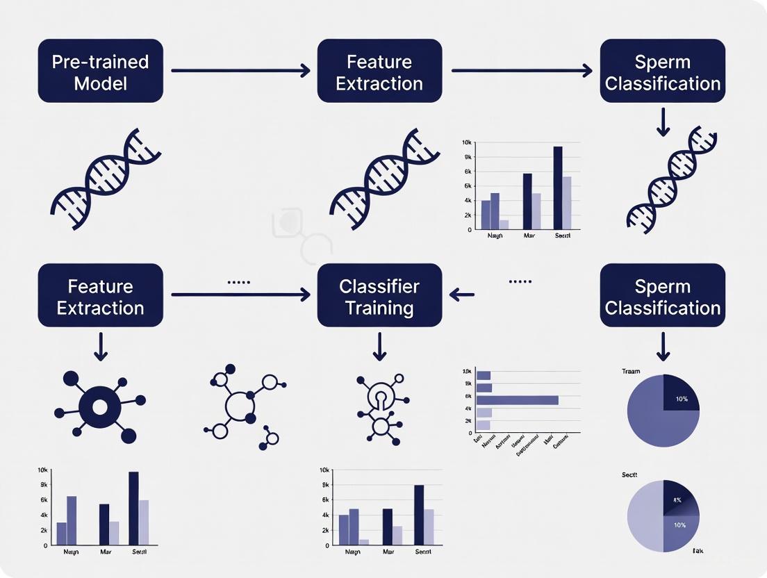
Workflow Visualization
Transfer Learning Workflow for Sperm Morphology Classification
Performance Metrics
The transfer learning approach detailed above has demonstrated exceptional performance in sperm morphology classification. When evaluated on the HuSHeM dataset, the modified AlexNet architecture achieved an average accuracy of 96.0% and precision of 96.4%, surpassing previous traditional machine learning and deep learning approaches [5]. Comparable transfer learning implementations using VGG16 architectures have achieved 94.1% accuracy on the same dataset, significantly exceeding conventional feature-based methods which showed accuracy rates between 58-62% on more challenging datasets [8].
The Scientist's Toolkit
Table 3: Essential Research Reagents and Computational Resources
| Category | Item/Resource | Specification/Function | Application Context |
|---|---|---|---|
| Datasets | HuSHeM Dataset | 216 sperm images; 4 morphology classes [5] | Algorithm training & validation |
| Datasets | SCIAN-MorphoSpermGS | 1854 sperm cell images; 5 expert-classified categories [8] | Benchmarking & comparison |
| Datasets | SMD/MSS Dataset | 1000+ images; David's modified classification [6] | Multi-class morphology assessment |
| Software | Python 3.8+ | With TensorFlow/PyTorch frameworks [6] | Deep learning implementation |
| Libraries | OpenCV | Image processing and augmentation [5] | Data preprocessing |
| Hardware | GPU-enabled Workstation | NVIDIA CUDA-compatible graphics cards | Model training acceleration |
| Staining | RAL Diagnostics Kit | Sperm staining for morphological clarity [6] | Sample preparation |
| Imaging | MMC CASA System | Computer-assisted semen analysis with camera [6] | Standardized image acquisition |
The escalating global burden of male infertility demands innovative approaches to diagnosis and analysis. Sperm morphology represents a critical diagnostic parameter that benefits significantly from computational approaches, particularly transfer learning methodologies. The experimental protocols outlined herein provide researchers with robust frameworks for implementing these advanced classification systems. Transfer learning techniques have demonstrated superior performance compared to traditional methods, achieving classification accuracy exceeding 96% in controlled assessments. As the field advances, the integration of these computational tools with standardized epidemiological data offers promising avenues for addressing male infertility through improved diagnostic precision, resource optimization in healthcare systems, and ultimately, enhanced clinical outcomes for affected individuals worldwide.
Sperm morphology assessment is a cornerstone of male fertility evaluation, providing critical diagnostic and prognostic information. Despite its clinical importance, the manual analysis of sperm shape, as outlined by the World Health Organization (WHO), remains plagued by significant inherent limitations. This application note details the core issues of subjectivity and poor reproducibility that undermine conventional manual assessment. Furthermore, it positions these challenges within the context of modern andrology laboratories, where automated solutions, particularly those leveraging transfer learning for sperm classification, are emerging as viable solutions to standardize and enhance diagnostic accuracy.
The Core Challenge: Subjectivity and Variability
The fundamental limitation of manual sperm morphology assessment lies in its reliance on the visual interpretation of a technologist. This process is inherently subjective, leading to substantial inter- and intra-observer variability. The complexity of the task—requiring the simultaneous evaluation of the head, midpiece, and tail against multiple strict criteria—makes consistent application of rules challenging, even among seasoned experts.
Quantitative Evidence of Inter-Expert Disagreement
Recent studies provide stark quantitative evidence of this variability. An analysis of inter-expert agreement in sperm cell classification revealed a concerning distribution: total agreement (TA) among three experts occurred in only 41% of cases, while partial agreement (PA) was seen in 35%, and no agreement (NA) was found in 24% of the spermatozoa analyzed [6]. This indicates that for nearly a quarter of sperm cells, three qualified experts could not concur on a classification.
External Quality Control (EQC) data over a six-year period (2015-2020) further highlights which specific morphological criteria are most prone to subjective interpretation. The table below summarizes the agreement levels for various WHO strict criteria among EQC participants [9].
Table 1: Variability in the Assessment of WHO Sperm Morphology Criteria Based on EQC Data (2015-2020)
| Morphological Criterion | Agreement Level | Agreement Percentage |
|---|---|---|
| Head Ovality | Poor | <60% |
| Regularity of Head Contour | Poor | <60% |
| Midpiece Regularity | Poor | <60% |
| Midpiece/Head Alignment | Poor | <60% |
| Acrosomal Region (40-70%) | Intermediate | 60-90% |
| Major Axes Alignment | Intermediate | 60-90% |
| Acrosomal Vacuoles (<20%) | Good | >90% |
| Excessive Residual Cytoplasm | Good | >90% |
| Tail Thinner than Midpiece | Good | >90% |
This data identifies head shape and midpiece contour/alignment as the primary sources of diagnostic inconsistency, whereas assessments of the acrosome, residual cytoplasm, and tail are more reliable [9].
Impact of Classification System Complexity
The level of disagreement is directly correlated with the complexity of the classification system used. A 2025 training study demonstrated that untrained morphologists showed significantly higher accuracy and lower variation when using a simple 2-category system (normal/abnormal) compared to more detailed systems [10].
Table 2: Classification Accuracy of Untrained Morphologists Across Different Systems
| Classification System | Number of Categories | Untrained User Accuracy |
|---|---|---|
| Normal/Abnormal | 2 | 81.0 ± 2.5% |
| Defect Location | 5 | 68.0 ± 3.6% |
| Specific Defect Types | 8 | 64.0 ± 3.5% |
| Granular Defect Types | 25 | 53.0 ± 3.7% |
This demonstrates a clear inverse relationship between system complexity and consensus, underscoring the difficulty in standardizing manual assessment across laboratories that may use different classification schemes [10].
Experimental Protocols for Investigating Assessment Variability
To quantify and address these limitations, researchers can employ the following experimental protocols.
Protocol 1: Quantifying Inter-Observer Variability
This protocol measures the degree of disagreement between different analysts within a laboratory.
- Sample Preparation: Prepare semen smears from at least 10 different patient samples using the Papanicolaou (PAP) staining method, as recommended by the WHO [11] [9].
- Image Acquisition: Acquire a minimum of 200 high-quality, digitized images of individual spermatozoa per sample using a bright-field microscope with a 100x oil immersion objective [6] [11].
- Blinded Assessment: Have at least three trained morphologists independently classify each sperm image according to a predefined system (e.g., the modified David classification with 12 classes or WHO strict criteria) [6] [9].
- Data Analysis: Calculate the percentage agreement for each morphological category. Use statistical measures such as Fleiss' Kappa to quantify the level of inter-observer agreement beyond what would be expected by chance [6].
Protocol 2: Evaluating the Impact of Training on Reproducibility
This protocol assesses whether standardized training can improve consistency among novice morphologists.
- Recruitment: Recruit a cohort of novice morphologists (n=16-22) with no prior experience in sperm morphology assessment [10].
- Baseline Testing: Administer a baseline test using a dataset of expert-validated sperm images across multiple classification systems (e.g., 2, 5, 8, and 25 categories) to establish initial accuracy and speed [10].
- Structured Training: Implement a training intervention using a standardized tool, such as the "Sperm Morphology Assessment Standardisation Training Tool," which employs machine learning principles and expert consensus "ground truth" labels [10].
- Post-Training Evaluation: Conduct repeated tests over a period of several weeks to monitor improvements in accuracy and diagnostic speed. Compare post-training results with baseline performance to quantify the effect of standardized training [10].
The Pathway to Standardization: AI and Transfer Learning
The documented limitations of manual assessment have accelerated the development of automated solutions. Artificial Intelligence (AI), particularly deep learning, offers a path toward objective, standardized, and high-throughput sperm morphology analysis [6] [7] [12].
The Role of Transfer Learning in Sperm Classification
A significant challenge in developing robust AI models is the scarcity of large, high-quality, annotated datasets of sperm images [7] [13]. Transfer learning is a powerful technique that addresses this bottleneck. It involves taking a pre-trained deep learning model (e.g., AlexNet, ResNet)—already skilled at feature extraction from a vast general image database like ImageNet—and fine-tuning it for the specific task of sperm classification [5]. This approach reduces computational costs, saves time, and achieves high accuracy even with limited medical image datasets [5].
Experimental Protocol: Implementing a Transfer Learning Approach
This protocol outlines the key steps for developing a sperm classifier using transfer learning.
- Data Curation: Collect or obtain a dataset of sperm images with expert-annotated ground truth labels. Publicly available datasets such as HuSHeM or SCIAN can be used for this purpose [5].
- Data Preprocessing: Clean and preprocess the images. This includes resizing images to the input dimensions of the pre-trained model, normalization, and data augmentation techniques (e.g., rotation, flipping, brightness/contrast adjustment) to increase dataset diversity and improve model robustness [6] [5] [14].
- Model Selection and Adaptation: Select a pre-trained Convolutional Neural Network (CNN) architecture like AlexNet or ResNet. Modify the final classification layer to match the number of sperm morphology classes in your dataset (e.g., 4 classes: normal, tapered, pyriform, amorphous) [5].
- Model Training (Fine-Tuning): Train the model on your sperm image dataset. Initially, freeze the weights of the early layers (which detect general features) and only train the later, task-specific layers. This preserves general feature knowledge while adapting the model to the new task [5].
- Validation and Testing: Evaluate the model's performance on a separate, unseen test set of images. Report standard metrics such as accuracy, precision, recall, and F1-score to benchmark its performance against manual assessment [5].
The Scientist's Toolkit: Research Reagent Solutions
The following table details key reagents and materials essential for conducting standardized sperm morphology research, whether for manual assessment or the development of AI-based models.
Table 3: Essential Research Reagents and Materials for Sperm Morphology Analysis
| Reagent / Material | Function / Application | Specifications / Standards |
|---|---|---|
| Papanicolaou (PAP) Stain | Standard staining for sperm morphology; allows clear differentiation of head, acrosome, midpiece, and tail. | Recommended as the reference staining method by WHO and ISO 23162 [11] [9]. |
| RAL Diagnostics Stain | A standardized staining kit used for sperm morphology assessment as an alternative to PAP. | Used in developing the SMD/MSS dataset for deep learning model training [6]. |
| SSA-II Plus CASA System | Computer-Assisted Semen Analysis system for automated image acquisition and morphometric parameter measurement. | Used for high-throughput data collection and to provide objective measurements of head length, width, area, etc. [11]. |
| Expert-Validated Datasets | Publicly available image datasets with "ground truth" labels for training and validating AI models. | Examples: HuSHeM (216 images), SCIAN (1854 images), VISEM-Tracking (656k+ annotations) [7] [13] [5]. |
| Pre-trained CNN Models | Deep learning models (e.g., AlexNet, ResNet, U-Net) pre-trained on large image datasets. | Serves as the foundation for transfer learning, significantly reducing development time and data requirements for sperm classification tasks [5] [14]. |
The subjectivity and poor reproducibility of manual sperm morphology assessment are well-documented, quantifiable problems that compromise diagnostic consistency. These limitations are primarily driven by inter-observer variability and the complexity of classification systems. The integration of AI, specifically deep learning with transfer learning, presents a transformative solution. By leveraging pre-trained models and standardized protocols, researchers and clinicians can overcome data scarcity and develop robust, automated systems. This shift towards computational andrology promises to deliver the objective, reproducible, and high-throughput analysis necessary for advanced male fertility diagnostics and research.
Within the broader scope of research on transfer learning for sperm classification, it is crucial to understand the foundations and limitations of the methods it aims to supersede. Conventional machine learning (ML) has played a pivotal role in automating sperm morphology analysis, a critical diagnostic procedure for male infertility where male factors contribute to approximately 50% of cases [13] [7]. These traditional algorithms sought to introduce objectivity and consistency into an process traditionally burdened by high inter-observer variability and subjectivity [13] [6].
The defining characteristic of these conventional ML approaches is their fundamental reliance on handcrafted features. This methodology depends on manual image analysis and the extraction of specific, pre-defined characteristics—such as shape, texture, and grayscale intensity—before these features are fed into a classifier [13] [5]. This document details the standard protocols for building such models, quantitatively summarizes their performance, and analyzes the inherent pitfalls of this paradigm, thereby framing the rationale for the shift towards deep learning and transfer learning in modern sperm classification research.
Experimental Protocols & Workflows
The development of a conventional ML model for sperm morphology analysis follows a standardized, multi-stage pipeline. The workflow is fundamentally sequential, where the output of each stage directly influences the success of the next.
Protocol: Traditional Sperm Image Analysis via Handcrafted Features
Objective: To classify human sperm cells into morphological categories (e.g., normal, tapered, pyriform, amorphous) using a conventional machine learning pipeline based on manually engineered features.
Sample Preparation and Data Acquisition
- Sample Collection & Staining: Collect semen samples and prepare smears following World Health Organization (WHO) guidelines. Stain slides using a commercially available staining kit (e.g., RAL Diagnostics kit or Diff-Quik method) to enhance cellular contrast [6] [5].
- Image Acquisition: Capture digital images of individual spermatozoa using an optical microscope equipped with a digital camera, typically with a 100x oil immersion objective in bright-field mode [6] [5]. Systems like the MMC Computer-Assisted Semen Analysis (CASA) system can be used for this purpose.
Image Pre-processing and Manual Feature Engineering
- Goal: Isolate the sperm head and extract descriptive numerical features.
- Steps:
- Denoising: Apply filters (e.g., wavelet denoising, low-pass filters) to reduce background noise and enhance the sperm signal [15] [5].
- Conversion to Monochrome: Transform RGB images to grayscale to simplify subsequent analysis [5].
- Sperm Head Segmentation:
- Apply edge detection operators (e.g., Sobel operator) to highlight sperm contours [5].
- Use adaptive thresholding algorithms to create a binary image separating the sperm head from the background [5].
- Perform morphological operations (erosion and dilation) to eliminate small interference spots and smooth the contour [5].
- Employ clustering algorithms like K-means to isolate the sperm head based on color or intensity [13] [7].
- Contour Analysis & Feature Extraction: Fit an ellipse to the sperm head contour to determine its major and minor axes. This allows for cropping and rotational alignment to a uniform direction [5].
- Manual Feature Extraction: This is the core, hands-on engineering step. Extract the following types of features from the processed sperm head image:
Model Training and Classification
- Dataset Partitioning: Randomly split the dataset of extracted feature vectors into a training subset (e.g., 80%) and a testing subset (e.g., 20%) [6].
- Classifier Training: Train a selected classifier on the training feature vectors and their corresponding morphological labels (provided by expert embryologists).
- Model Evaluation: Use the held-out testing set to evaluate the final model's performance using metrics such as accuracy, precision, recall, and area under the curve (AUC) [6] [15].
The following diagram illustrates this multi-stage workflow, highlighting its sequential and engineered nature.
Performance Data and Pitfalls
The conventional ML pipeline has demonstrated variable but ultimately limited success in research settings. The table below summarizes the performance of several representative approaches, highlighting the algorithms and datasets used.
Table 1: Performance of Conventional Machine Learning Models in Sperm Morphology Analysis
| Study Citation | ML Algorithm(s) Used | Key Handcrafted Features | Reported Performance | Noted Limitations |
|---|---|---|---|---|
| Bijar A et al. [7] | Bayesian Density Estimation | Shape-based descriptors (Hu moments, Zernike moments, Fourier descriptors) | 90% accuracy (4-class head classification) | Relies exclusively on shape; lacks texture/grayscale data [7]. |
| Mirsky SK et al. [7] | Support Vector Machine (SVM) | Unspecified sperm head features | AUC-ROC: 88.59%, Precision >90% | Binary classification (good/bad) only [7]. |
| Chang V et al. [7] | Fourier Descriptor + SVM | Fourier shape descriptors | 49% accuracy (non-normal head classification) | Highlights high inter-expert variability and task difficulty [7]. |
| Shaker F et al. [5] | Adaptive Patch-based Dictionary Learning | Image patches from sperm heads | Avg. True Positive Rate: 62% (SCIAN dataset) | Requires manual feature extraction, not end-to-end [5]. |
Critical Analysis of Pitfalls
The data in Table 1 reveals several fundamental pitfalls inherent to the handcrafted feature approach:
Limited Scope and Granularity: Most conventional models are restricted to classifying sperm heads into a small number of categories (e.g., normal, tapered, pyriform, amorphous) [7] [5]. They generally fail to address the complete sperm structure, ignoring critical diagnostic information from the neck, midpiece, and tail, which according to WHO standards, encompasses 26 types of abnormal morphology [13] [7].
Inadequate Generalization and Accuracy: The performance of these models is highly variable and often unsatisfactory for clinical application. As shown in Table 1, accuracy can be as low as 49% on more challenging classification tasks, a figure that reflects the high inter-expert variability in the field [7]. These algorithms also struggle to distinguish sperm heads from impurities and cellular debris in semen samples, leading to misclassification [7].
Technical Drawbacks: The reliance on manually set thresholds and texture features frequently results in over-segmentation or under-segmentation [7]. Furthermore, the process of manual feature extraction is not only cumbersome and time-consuming but also inherently limits the algorithm's generalization ability. A feature set tuned for one dataset often performs poorly on another, as it cannot learn new, relevant features on its own [7].
The Scientist's Toolkit
Table 2: Essential Research Reagents and Computational Tools for Conventional ML in Sperm Analysis
| Item / Resource | Type | Function / Description | Example / Citation |
|---|---|---|---|
| SCIAN-MorphoSpermGS | Public Dataset | A gold-standard dataset with 1,854 sperm images for training and evaluating models, classified into five categories. | [7] [5] |
| HuSHeM | Public Dataset | A publicly available dataset containing 216 human sperm head images across four morphological classes. | [15] [5] |
| RAL Diagnostics Staining Kit | Laboratory Reagent | Used for staining semen smears to enhance contrast and morphological detail for microscopic imaging. | [6] |
| Support Vector Machine (SVM) | Computational Algorithm | A robust classifier frequently used as the final step in the pipeline to categorize sperm based on engineered features. | [7] [16] |
| K-means Clustering | Computational Algorithm | An unsupervised algorithm commonly used for segmenting and isolating the sperm head from the image background. | [13] [7] |
| Shape Descriptors (Hu, Zernike) | Computational Feature | Mathematical representations of shape and contour used as handcrafted features for the classifier. | [7] [15] |
Conventional machine learning, built on a foundation of handcrafted features, established the initial pathway toward automated sperm morphology analysis. The experimental protocols and performance data detailed herein underscore both its historical contribution and its profound limitations. The paradigm's reliance on manual feature engineering results in models with restricted classification granularity, inconsistent performance, and poor generalizability.
These identified pitfalls provide the critical context and justification for the ongoing research shift towards deep learning and, more specifically, transfer learning. Deep learning models, with their ability to automatically learn hierarchical and discriminative features directly from raw pixel data, represent a necessary evolution to overcome the constraints outlined in this document and build more robust, accurate, and clinically viable automated sperm analysis systems.
In the field of male infertility research, sperm morphology analysis is a crucial diagnostic procedure. The application of deep learning, particularly transfer learning, to automate and standardize this analysis shows significant promise [17]. However, the development of robust, generalizable models is fundamentally constrained by a critical bottleneck: the lack of standardized, high-quality annotated datasets [13]. This Application Note details this central challenge, quantitatively summarizes existing data resources, and provides detailed protocols for dataset creation to empower research in transfer learning for sperm classification.
The Core Dataset Challenge
Deep learning models require large volumes of high-quality, consistently annotated data to train effectively. In sperm morphology analysis, this requirement is difficult to meet for several key reasons:
- Inherent Data Complexity and Subjectivity: Sperm defect assessment requires the simultaneous evaluation of the head, vacuoles, midpiece, and tail, which substantially increases annotation difficulty and complexity [13]. The process is inherently subjective, leading to significant inter-observer variability even among experts, with reported kappa values as low as 0.05–0.15 [15].
- Acquisition and Annotation Difficulties: Sperm may appear intertwined in images, or only partial structures may be displayed, complicating both automated and manual analysis [13]. The process of manual annotation is time-intensive and requires specialized expertise [15].
- Impact on Model Performance: Without standardized datasets, models trained on one dataset often fail to generalize well to images from different clinics or acquired under different conditions [13]. This limits their clinical applicability and robustness.
A Landscape of Existing Datasets and Performance
Numerous public and private datasets have been developed to address these needs. The table below summarizes key datasets, highlighting their characteristics and the performance benchmarks achieved by deep learning models on them.
Table 1: Summary of Key Sperm Morphology Datasets and Model Performance
| Dataset Name | Key Characteristics | Image Count (Original) | Annotation Type | Noted Limitations | Representative Model Performance |
|---|---|---|---|---|---|
| HuSHeM [13] [15] | Stained sperm heads, higher resolution | 725 (216 public) | Classification | Limited public availability, focuses only on heads | 96.77% accuracy with CBAM-enhanced ResNet50 & DFE [15] |
| SMIDS [13] [15] | Stained sperm images | 3,000 | Classification (3-class) | - | 96.08% accuracy with CBAM-enhanced ResNet50 & DFE [15] |
| MHSMA [13] [18] | Non-stained, grayscale sperm heads | 1,540 | Classification | No-stain, noisy, low resolution [13] | Used for deep learning model development [18] |
| VISEM-Tracking [13] | Low-resolution unstained sperm and videos | 656,334 annotated objects | Detection, Tracking, Regression | Low-resolution, unstained [13] | A multi-modal dataset for sperm analysis tasks [13] |
| SVIA [13] [18] [19] | Low-resolution unstained sperm and videos | 4,041 images; 125,000 annotated instances | Detection, Segmentation, Classification | Low-resolution, unstained [13] | Used for training segmentation models like Mask R-CNN [19] |
| SMD/MSS [6] | Stained sperm, based on David classification | 1,000 (extended to 6,035 via augmentation) | Classification (12 defect classes) | - | Deep learning model accuracy ranged from 55% to 92% [6] |
A comparative analysis of state-of-the-art deep learning models further illustrates the interplay between data and architecture. The following table synthesizes quantitative results from recent studies.
Table 2: Performance of Deep Learning Models on Sperm Morphology Tasks
| Model / Framework | Primary Task | Dataset Used | Key Metric | Performance |
|---|---|---|---|---|
| CBAM-ResNet50 with DFE [15] | Head Morphology Classification | SMIDS | Accuracy | 96.08% |
| CBAM-ResNet50 with DFE [15] | Head Morphology Classification | HuSHeM | Accuracy | 96.77% |
| In-house AI (ResNet50) [18] | Unstained Live Sperm Morphology | Novel Confocal Microscopy Dataset | Correlation with CASA | r = 0.88 |
| Mask R-CNN [19] | Multi-part Segmentation (Head, Nucleus, Acrosome) | Live Unstained Sperm Dataset | IoU | Outperformed YOLOv8 & YOLO11 |
| U-Net [19] | Multi-part Segmentation (Tail) | Live Unstained Sperm Dataset | IoU | Highest performance for tail segment |
| CNN with Augmentation [6] | Multi-class Defect Classification | SMD/MSS | Accuracy | 55% - 92% (varies by class) |
Detailed Experimental Protocols
To facilitate the creation of high-quality datasets, we outline two detailed experimental protocols from recent literature.
Protocol 1: Creating a High-Resolution Unstained Sperm Dataset for Transfer Learning
This protocol is adapted from a 2025 study that used confocal microscopy to create a high-quality dataset for training an AI model to assess unstained, live sperm [18]. This is particularly valuable for clinical applications where staining is undesirable.
1. Sample Preparation
- Participants: Enroll donors following ethical guidelines. Maintain sexual abstinence for 2-7 days prior to sample collection [18].
- Liquefaction: Check semen samples within 30 minutes of ejaculation. Preserve specimens at 37°C before and during analysis [18].
- Slide Preparation: Dispense a 6 µL droplet onto a standard two-chamber slide with a depth of 20 µm [18].
2. Image Acquisition via Confocal Microscopy
- Microscope: Use a Confocal Laser Scanning Microscope (e.g., LSM 800) [18].
- Settings: Set magnification to 40x in confocal mode (LSM, Z-stack). Set Z-stack interval to 0.5 µm, covering a total range of 2 µm. Use a frame time of ~633 ms and an image size of 512 x 512 pixels [18].
- Data Collection: Capture at least 200 sperm images per sample, with each capture containing 2-3 sperm [18].
3. Expert Annotation and Categorization
- Annotation Tool: Use a program like LabelImg to manually draw bounding boxes around each sperm [18].
- Criteria for Normal Sperm: Based on WHO guidelines, classify sperm as normal if they have a smooth oval head (length-to-width ratio of 1.5–2), no vacuoles, a slender/regular neck, and a uniform tail [18].
- Categorization: Categorize each sperm image into normal or abnormal datasets. Abnormal sperm are characterized by defects in the head (tapered, amorphous, pyriform, round), observable vacuoles, aberrant neck, or abnormal tail [18].
4. Model Training with Transfer Learning
- Model Selection: Choose a pre-trained model such as ResNet50 for image classification tasks [18].
- Training: Train the model on the annotated dataset to minimize the difference between predicted and actual labels. A study using this method reported a test accuracy of 93% after 150 epochs [18].
Protocol 2: Building an Augmented Dataset for Multi-Class Defect Classification
This protocol, based on the creation of the SMD/MSS dataset, focuses on using data augmentation to balance morphological classes and train a model for detailed defect classification according to the modified David classification [6].
1. Sample Preparation and Staining
- Sample Inclusion: Use samples with a sperm concentration of at least 5 million/mL. Exclude samples with high concentrations (>200 million/mL) to avoid image overlap [6].
- Smear Preparation and Staining: Prepare smears following WHO guidelines and stain with a Romanowsky stain variant (e.g., RAL Diagnostics kit) [6].
2. Data Acquisition and Expert Classification
- System: Use a Computer-Aided Semen Analysis (CASA) system (e.g., MMC) with an optical microscope equipped with a digital camera and a 100x oil immersion objective in bright field mode [6].
- Classification: Have each spermatozoon manually classified by three independent experts. The classification should follow a structured system like the modified David classification, which includes 12 classes of defects (e.g., 7 head defects, 2 midpiece defects, 3 tail defects) [6].
- Inter-Expert Agreement Analysis: Calculate the level of agreement among experts (e.g., Total Agreement: 3/3, Partial Agreement: 2/3, No Agreement: 0/3) using statistical tests like Fisher's exact test [6].
3. Data Augmentation and Pre-processing
- Augmentation Techniques: Apply techniques such as rotation, scaling, and flipping to augment the dataset size and balance the representation of different morphological classes. One study increased a dataset from 1,000 to 6,035 images using augmentation [6].
- Image Pre-processing: Resize images (e.g., to 80x80 pixels for grayscale) and normalize pixel values to bring them to a common scale [6].
4. Model Training and Evaluation
- Data Partitioning: Split the augmented dataset randomly, using 80% for training and 20% for testing [6].
- Algorithm Implementation: Develop a Convolutional Neural Network (CNN) algorithm using a framework like Python. Train the model on the training set and evaluate its performance on the unseen test set [6].
The Scientist's Toolkit: Essential Research Reagents and Materials
Table 3: Key Research Reagent Solutions for Sperm Morphology Analysis
| Item | Function / Application |
|---|---|
| RAL Diagnostics Staining Kit (Romanowsky-type stain) | Stains sperm cells on smears to provide contrast for visualizing morphological details under a light microscope [6]. |
| Diff-Quik Stain (Romanowsky stain variant) | Used for rapid staining of sperm for morphology assessment, typically in Computer-Aided Semen Analysis (CASA) [18]. |
| Leja Standard Two-Chamber Slides (20 µm depth) | Provides standardized chambers for preparing semen samples for microscopic analysis, ensuring consistent depth for imaging [18]. |
| Confocal Laser Scanning Microscope (e.g., Zeiss LSM 800) | Enables high-resolution, Z-stack image acquisition of live, unstained sperm at lower magnifications, preserving sperm viability [18]. |
| MMC or IVOS II CASA System | Automated system for acquiring and analyzing sperm images, used for measuring concentration, motility, and morphometric parameters [18] [6]. |
| LabelImg Program | An open-source graphical image annotation tool used to draw bounding boxes around sperm for creating ground truth data [18]. |
The field of artificial intelligence (AI) has undergone a fundamental transformation, moving from traditional, manually-engineered algorithms to sophisticated, data-driven learning systems. This paradigm shift is most evident in the application of Deep Learning (DL) and Transfer Learning (TL) to complex scientific domains, where they are revolutionizing how researchers extract information from data. Traditional machine learning approaches have long been hampered by their reliance on handcrafted features—where domain experts must manually identify and quantify relevant characteristics from raw data, a process that is both time-consuming and inherently biased by human perception [20].
Deep learning represents a radical departure from this tradition. As a subfield of machine learning, it utilizes artificial neural networks with multiple layers (hence "deep") to automatically learn hierarchical representations of data directly from raw inputs, such as images. This automatic feature extraction eliminates the need for manual feature engineering, allowing models to discover complex, non-linear patterns that may be imperceptible to human experts [7] [20]. However, the power of deep learning comes with significant requirements: it is notoriously "data-hungry," often needing thousands or even millions of labeled examples to perform effectively, and demands substantial computational resources, typically requiring high-end GPUs for training [20].
The critical innovation that bridges the gap between deep learning's potential and practical application in data-scarce scientific fields is transfer learning. TL addresses the fundamental challenge of limited dataset sizes in specialized domains by leveraging knowledge gained from solving one problem (typically on a large, general-purpose dataset) and applying it to a different but related problem. This approach allows researchers to bootstrap specialized models with minimal data by fine-tuning pre-trained networks, dramatically reducing both data requirements and training time while improving overall performance [5] [21]. Together, deep learning and transfer learning are creating a new paradigm for scientific discovery, enabling breakthroughs in fields from medical imaging to reproductive biology.
Technical Foundations
Deep Learning Architectures
At the heart of the deep learning revolution are several key neural network architectures, each with unique capabilities for processing different types of data:
Convolutional Neural Networks (CNNs): Specifically designed for processing grid-like data such as images, CNNs use a series of convolutional layers that act as learnable filters to detect hierarchical patterns—from simple edges and textures in early layers to complex object parts in deeper layers. This architecture is particularly effective for image classification, object detection, and segmentation tasks [6] [5]. The spatial hierarchy learned by CNNs makes them ideally suited for analyzing medical images, including sperm morphology.
Transformer Networks: Originally developed for natural language processing, transformers utilize an attention mechanism to weigh the importance of different parts of the input data when making predictions. This architecture has recently been adapted for tabular data through models like TabTransformer, which creates robust embeddings for categorical variables and demonstrates strong performance even with limited labeled data [22]. Transformers excel at capturing long-range dependencies in data, making them powerful for diverse scientific applications.
Siamese Networks: A specialized architecture for contrastive learning, Siamese networks consist of two or more identical subnetworks that process different inputs simultaneously, then compare their outputs to learn similarity metrics. This approach is particularly valuable for one-shot or few-shot learning scenarios where labeled examples are extremely scarce, such as detecting rare defects in industrial quality control or classifying unusual morphological variants [23].
The Transfer Learning Workflow
Transfer learning operationalizes knowledge transfer through a systematic workflow that maximizes learning efficiency:
Pre-training on Source Domain: A base model (typically a CNN like AlexNet, VGG, or ResNet) is first trained on a large-scale benchmark dataset such as ImageNet, which contains over a million images across thousands of categories [5] [21]. This phase requires substantial computational resources but needs to be done only once, as the learned feature representations—especially in the early layers—capture universal visual patterns like edges, shapes, and textures.
Knowledge Transfer: The pre-trained model's weights are imported, preserving the general feature extraction capabilities developed during pre-training. The architecture is typically modified by replacing the final classification layer(s) with new layers tailored to the target task (e.g., classifying sperm morphology into specific abnormality categories rather than generic object classes) [5].
Fine-tuning on Target Domain: The model is further trained (fine-tuned) on the specialized target dataset, allowing the weights to adapt to the specific characteristics of the new domain. Strategic approaches vary in how many layers are fine-tuned—options include updating only the new final layers while keeping earlier layers frozen, or progressively unfreezing layers with lower learning rates to balance specificity and generality [5] [21].
Application in Sperm Morphology Research
The Clinical Challenge
Infertility affects approximately 15% of couples globally, with male factors contributing to nearly 50% of cases [6] [7]. Sperm morphology analysis represents a crucial diagnostic procedure in male fertility assessment, as the shape and structure of spermatozoa are proven indicators of biological function and fertilization potential [6] [5]. Traditional manual morphological assessment is exceptionally challenging, characterized by:
- High subjectivity and variability between different technicians and laboratories [6] [7]
- Substantial time requirements for analyzing 200+ sperm cells per sample according to WHO standards [7]
- Classification complexity with up to 26 types of abnormalities across head, neck, and tail compartments [7]
- Disagreement among experts, with studies showing significant inter-observer variability in morphological classification [6]
These limitations of conventional analysis have created an pressing need for automated, objective, and standardized approaches that can deliver consistent, reproducible results across clinical settings.
Comparative Performance: Traditional ML vs. Deep Learning vs. Transfer Learning
The evolution of computational approaches for sperm morphology analysis demonstrates a clear trajectory of performance improvement, with transfer learning emerging as the most effective strategy, particularly given the limited dataset sizes typical in medical domains.
Table 1: Performance Comparison of Different Computational Approaches for Sperm Morphology Classification
| Methodological Approach | Key Characteristics | Reported Accuracy | Data Requirements | Limitations |
|---|---|---|---|---|
| Traditional Machine Learning (SVM, K-means, Decision Trees) | Relies on handcrafted features (shape, texture, size); expert-driven feature selection | 49%-90% [7] | Moderate (hundreds of samples) | Limited to pre-defined features; poor generalization; often only classifies head defects |
| Deep Learning from Scratch (CNN trained on target domain only) | Automatic feature extraction; end-to-end learning | 62%-94.1% [5] | Very high (thousands of labeled samples) | Computationally intensive; requires large datasets; risk of overfitting with small datasets |
| Transfer Learning (Pre-trained CNN fine-tuned on sperm images) | Leverages pre-trained features; adapts to target domain | Up to 96.0% [5] | Low (hundreds of samples sufficient) | Optimal performance depends on source-target domain similarity; requires careful fine-tuning strategy |
The quantitative superiority of transfer learning is exemplified by a 2021 study that modified AlexNet architecture with batch normalization layers and pre-trained parameters from ImageNet, achieving 96.0% accuracy on the HuSHeM dataset for sperm head classification—significantly outperforming both traditional machine learning methods and deep learning models trained from scratch [5]. This approach demonstrated not only higher accuracy but also greater computational efficiency, with parameter counts less than one-sixth of a VGG16-based approach [5].
Experimental Protocol: Transfer Learning for Sperm Morphology Classification
For researchers implementing transfer learning for sperm classification, the following detailed protocol provides a robust methodological framework:
Data Acquisition and Preprocessing
Sample Preparation: Prepare semen smears following WHO laboratory guidelines [6]. Stain using standardized protocols (e.g., RAL Diagnostics staining kit or Diff-Quik method) to ensure consistent imaging characteristics [6] [5].
Image Acquisition: Capture individual sperm images using a Computer-Assisted Semen Analysis (CASA) system with a 100x oil immersion objective in bright-field mode [6]. Ensure each image contains a single spermatozoon with clear visibility of head, midpiece, and tail structures.
Expert Annotation: Have each sperm image independently classified by multiple experienced embryologists according to standardized classification systems (WHO criteria or modified David classification) [6] [5]. Resolve disagreements through consensus review with additional experts. A minimum of three expert annotations per image is recommended for establishing reliable ground truth.
Data Preprocessing Pipeline:
- Cropping: Automatically crop sperm heads using contour detection and elliptical fitting to focus on the most discriminative region [5].
- Rotation: Align sperm heads to a uniform orientation (e.g., major axis horizontal) to reduce rotational variance [5].
- Resizing: Standardize image dimensions to match input requirements of pre-trained models (typically 64×64 to 224×224 pixels) [5].
- Normalization: Scale pixel values to standard range (e.g., 0-1) using dataset mean and standard deviation.
Data Augmentation: Apply limited, realistic transformations to increase dataset diversity while preserving morphological integrity: slight rotations (±5°), minimal horizontal/vertical shifts (±10%), and careful brightness adjustments [6]. Avoid aggressive transformations that may alter morphological characteristics.
Transfer Learning Implementation
Model Selection: Choose appropriate pre-trained architecture based on dataset size and computational resources. For smaller datasets (<1000 images), AlexNet or EfficientNetB0 are recommended; for larger datasets, ResNet50 or VGG16 may be suitable [5] [21].
Architecture Modification:
Fine-tuning Strategy:
- Phase 1: Freeze all pre-trained layers and train only the newly added classification layers for 20-30 epochs with a reduced learning rate (e.g., 0.001).
- Phase 2: Unfreeze and fine-tune deeper layers of the network with an even lower learning rate (e.g., 0.0001) for an additional 30-50 epochs.
- Use early stopping with a patience of 10-15 epochs to prevent overfitting.
Training Configuration:
- Optimizer: Adam with default parameters (beta1=0.9, beta2=0.999)
- Loss Function: Categorical cross-entropy for multi-class classification
- Batch Size: 16-32 depending on available GPU memory
- Validation Split: 15-20% of training data for monitoring generalization performance
Model Evaluation
Performance Metrics: Compute comprehensive metrics including accuracy, precision, recall, F1-score, and area under the ROC curve (AUC) for each morphological class [5] [21].
Cross-Validation: Implement k-fold cross-validation (k=5 or 10) to obtain robust performance estimates and reduce variance from data partitioning [5].
Statistical Validation: Perform bootstrap resampling to calculate confidence intervals for performance metrics and ensure statistical significance of results [23].
Clinical Validation: Compare model classifications with independent expert annotations not used in training to assess real-world clinical relevance and diagnostic agreement.
Research Reagent Solutions
Successful implementation of deep learning for sperm morphology analysis requires both computational resources and specialized experimental materials:
Table 2: Essential Research Reagents and Resources for Sperm Morphology Analysis
| Resource Category | Specific Examples | Function/Application |
|---|---|---|
| Staining Kits | RAL Diagnostics kit, Diff-Quik method | Standardized staining of semen smears for consistent morphological visualization |
| Public Datasets | HuSHeM (216 images), SCIAN-MorphoSpermGS (1854 images), SMD/MSS (1000+ images), SVIA dataset (125,000+ annotations) [6] [7] [5] | Benchmarking algorithms; training and validation of models; comparative studies |
| Image Acquisition Systems | CASA (Computer-Assisted Semen Analysis) systems with digital cameras [6] | Standardized capture of sperm images under consistent magnification and lighting |
| Deep Learning Frameworks | TensorFlow, PyTorch, Keras with pre-trained models (AlexNet, VGG, ResNet, EfficientNet) [5] [21] | Implementation of transfer learning pipelines; model training and inference |
| Computational Infrastructure | GPU-accelerated workstations (NVIDIA RTX series or equivalent), cloud computing platforms | Handling computational demands of deep learning model training and evaluation |
Visualizing the Workflow
The following diagram illustrates the complete transfer learning workflow for sperm morphology classification, from data preparation through to model deployment:
Diagram 1: Complete transfer learning workflow for sperm morphology classification, showing knowledge transfer from general image recognition to specialized medical image analysis.
The paradigm shift represented by deep learning and transfer learning continues to evolve, with several emerging trends poised to further transform sperm morphology research and other biomedical applications:
Foundation models for tabular data, such as TabPFN, demonstrate that the transfer learning paradigm can extend beyond image data to structured clinical information, potentially enabling integrated analysis of both visual morphological data and associated clinical parameters [24]. Hybrid approaches combining the strengths of Contrastive Learning (CL) and Deep Transfer Learning (DTL) show promise for addressing extreme class imbalance situations, such as when certain morphological defects are exceptionally rare in patient populations [23]. Additionally, explainable AI techniques are being developed to address the "black box" nature of deep learning models, making their decision processes more interpretable to clinicians and researchers [22].
In conclusion, the integration of deep learning with transfer learning has fundamentally reshaped the landscape of sperm morphology analysis and biomedical research more broadly. This paradigm shift from manual feature engineering to automated, data-driven learning has enabled unprecedented accuracy in classification tasks while simultaneously addressing the critical challenge of limited dataset sizes in specialized medical domains. As these technologies continue to mature and become more accessible, they hold the potential to standardize and automate male fertility assessment globally, reducing inter-laboratory variability and providing clinicians with more reliable diagnostic information. The methodological framework presented in this article provides researchers with a comprehensive foundation for leveraging these transformative technologies in their own work, contributing to the ongoing advancement of computational approaches in reproductive medicine and beyond.
Implementing Transfer Learning Models for Sperm Classification: Architectures and Workflows
The manual assessment of sperm morphology is a cornerstone of male infertility diagnosis, yet it remains highly subjective, challenging to standardize, and dependent on the technician's expertise [25] [7]. Artificial intelligence (AI), particularly deep learning, offers a path toward automation, standardization, and improved accuracy in this critical area of reproductive medicine [6] [7]. However, a significant challenge in developing robust deep learning solutions is the frequent scarcity of large, annotated medical image datasets [25] [6].
Transfer learning has emerged as a powerful technique to overcome this data limitation [26]. This approach involves taking a model pre-trained on a very large dataset, such as ImageNet, and adapting it to a new, specific task—like sperm classification [27]. By leveraging the generic feature detectors (e.g., for edges, textures, shapes) learned from millions of images, researchers can achieve high performance on specialized medical tasks with limited data, saving substantial computational resources and time [26] [28]. This document provides a structured review of popular pre-trained architectures and detailed experimental protocols to guide researchers in selecting and implementing the most suitable model for sperm morphology analysis.
A Review of Popular Pre-trained Architectures
The selection of an appropriate pre-trained model is a critical first step. The following section reviews key architectures, highlighting their core innovations, strengths, and weaknesses in the context of biomedical image analysis.
Model Architectures: From AlexNet to ResNet
AlexNet (2012): A pioneering deep convolutional neural network that demonstrated the power of deep learning on a large scale by winning the ImageNet challenge in 2012 [29] [30]. Its key innovations included the use of the ReLU activation function to speed up training, and dropout layers to reduce overfitting [29] [30]. While foundational, its use of large filters (11x11, 5x5) and lower depth make it less efficient and performant compared to more modern architectures for complex tasks like sperm segmentation [29] [31].
VGG (VGG16 & VGG19) (2014): The VGG network family emphasized the importance of network depth by using a very uniform architecture built from stacks of small 3x3 convolutional filters [29] [31] [30]. This design increased depth and non-linearity while controlling the number of parameters, leading to significantly improved accuracy over AlexNet [31]. VGG's simple and consistent structure has made it a popular choice for feature extraction in transfer learning [31]. A primary drawback is its computational expense; the model has a large number of parameters, and the trained VGG16 model is over 500MB, making it potentially cumbersome for some deployment scenarios [29].
GoogleNet (Inception v1) (2014): This architecture introduced the "Inception module," which allowed the network to be wider rather than just deeper [29]. Its key innovation was using parallel convolution paths with filters of different sizes (1x1, 3x3, 5x5) within the same layer, enabling the efficient capture of features at multiple scales [29] [30]. Crucially, it used 1x1 convolutions for dimensionality reduction, which helped control computational cost [29]. This efficient design was a precursor to more complex and powerful modern networks.
ResNet (2015): The Residual Network (ResNet) addressed a fundamental problem in very deep networks: degradation. As networks become deeper, accuracy can saturate and then degrade, not due to overfitting but because of optimization difficulties [30]. ResNet introduced "skip connections" or residual connections that allow a layer to bypass the next layer, making it easier to train networks with hundreds or even thousands of layers [30]. This architecture mitigates the vanishing gradient problem and has become a default choice for many computer vision tasks due to its robustness and high performance [26] [30].
Comparative Analysis of Architectures
Table 1: Comparative analysis of popular pre-trained model architectures.
| Architecture | Key Innovation | Depth (Layers) | Strengths | Weaknesses / Suitability for Sperm Analysis |
|---|---|---|---|---|
| AlexNet [29] [30] | ReLU, Dropout, GPU Training | 8 | • Pioneering architecture• Proven effectiveness on ImageNet | • Lower depth and performance vs. newer models• Less suitable for fine-grained sperm feature extraction |
| VGG16/VGG19 [29] [31] | Depth with small (3x3) filters | 16 / 19 | • Simple, uniform architecture• High accuracy, excellent for feature extraction | • Very large model size (>500MB) [29]• Computationally expensive• Good candidate if resources allow |
| GoogleNet [29] [30] | Inception modules (multi-scale) | 22 | • Captures features at multiple scales• Computationally efficient | • More complex architecture• Potential for fine-grained multi-scale sperm analysis (head, tail) |
| ResNet [26] [30] | Residual (skip) connections | 50, 101, 152+ | • Solves degradation in very deep networks• Robust training, state-of-the-art performance | • Often the preferred starting point for its balance of depth and trainability |
Experimental Protocols for Sperm Morphology Analysis
This section outlines a standardized experimental workflow for applying pre-trained models to sperm morphology analysis, from data preparation to model evaluation.
Workflow for Transfer Learning in Sperm Analysis
The following diagram visualizes the end-to-end experimental protocol for applying transfer learning to sperm classification.
Transfer Learning Workflow for Sperm Analysis
Data Preparation and Augmentation Protocol
Objective: To create a robust and generalized dataset for training a deep learning model, mitigating the risk of overfitting given the typically limited data available [25] [6].
Data Acquisition:
- Acquire sperm images using a Computer-Assisted Semen Analysis (CASA) system or a microscope with a digital camera [6]. Standardize the staining process (e.g., modified Hematoxylin/Eosin) and use an oil immersion 100x objective for consistent, high-quality images [25] [6].
- Annotation: Each sperm image must be meticulously annotated by multiple experts to establish a reliable ground truth. This involves labeling different morphological parts (head, acrosome, nucleus, midpiece, tail) and classifying them according to a standard like the modified David classification [6]. Analyze inter-expert agreement (e.g., Total Agreement, Partial Agreement) to quantify the subjectivity of the task and ensure label quality [6].
Data Preprocessing:
- Cleaning: Identify and handle any missing or corrupt images.
- Normalization: Resize all images to the input dimensions required by the chosen pre-trained model (e.g., 224x224 for VGG) [31]. Normalize pixel values to a standard range, typically [0, 1] or [-1, 1].
- Denoising: Apply techniques to reduce noise from insufficient lighting or poor staining, which can improve model performance [6].
Data Augmentation (Critical Step):
- To artificially expand the dataset and improve model generalization, apply a series of random transformations to the training images. Recommended techniques include [25] [6]:
- Geometric: Random rotation (±10°), horizontal and vertical flipping, slight zooming (±10%), and shearing.
- Photometric: Adjusting brightness, contrast, and saturation within a small range (±20%).
- Implementation: This is typically performed in real-time during training using frameworks like TensorFlow/Keras or PyTorch.
- To artificially expand the dataset and improve model generalization, apply a series of random transformations to the training images. Recommended techniques include [25] [6]:
Transfer Learning and Model Training Protocol
Objective: To adapt a pre-trained model to the specific task of sperm morphology classification or segmentation.
Model Selection & Adaptation:
- Selection: Choose a pre-trained model (see Section 2). ResNet-based models are often a strong starting point due to their trainability [30].
- Adaptation: Remove the original classification head (the final fully-connected layer) of the pre-trained model. Replace it with a new, untrained head tailored to the sperm classification task. This could be a simple softmax layer for binary (normal/abnormal) classification or multiple output layers for a multi-label problem [27].
Training Strategies:
- Feature Extraction: Freeze the weights of all convolutional layers from the pre-trained model. Only train the weights of the newly added classification head. This is a fast, computationally cheap method suitable for very small datasets [27].
- Fine-Tuning: After feature extraction, unfreeze some of the deeper layers of the pre-trained model and jointly train them with the new head. This allows the model to adapt its more specialized features to the sperm image domain, potentially leading to higher performance [27] [28]. Use a lower learning rate (e.g., 10 times smaller) for the fine-tuned layers to avoid destructive updates to the pre-trained weights [27].
Training Configuration:
- Optimizer: Use optimizers like Stochastic Gradient Descent (SGD) with momentum (e.g., 0.9) or Adam [29] [27].
- Learning Rate: Employ a learning rate scheduler to reduce the rate when validation performance plateaus (e.g., reduce by a factor of 10 every 10 epochs) [29].
- Regularization: Utilize dropout layers in the fully-connected layers to prevent overfitting [29] [27].
Model Evaluation and Validation Protocol
Objective: To rigorously assess the model's performance and ensure its generalizability to new, unseen data.
- Data Splitting: Split the annotated dataset into three subsets: Training Set (~70-80%), Validation Set (~10-15%), and Test Set (~10-15%) [6]. The test set must be held back and used only for the final evaluation.
- Evaluation Metrics: Move beyond simple accuracy. Report a comprehensive set of metrics calculated on the test set [32]:
- Precision: The ability of the classifier not to label a negative sample as positive.
- Recall (Sensitivity): The ability of the classifier to find all the positive samples.
- F1-Score: The harmonic mean of precision and recall.
- Confusion Matrix: A detailed breakdown of the model's predictions versus the actual labels.
- Comparative Analysis: Benchmark the performance of the transfer learning approach against custom-built models (e.g., a simple CNN) or traditional machine learning methods (e.g., SVM with handcrafted features) to quantify the benefits [32] [7].
The Scientist's Toolkit: Essential Research Reagents & Materials
Table 2: Key reagents, materials, and computational tools for deep learning-based sperm analysis.
| Item Name | Function / Explanation | Example / Specification |
|---|---|---|
| CASA System [6] | For standardized, high-throughput acquisition of digital sperm images. | MMC CASA system or equivalent. |
| Standardized Staining Kit [6] | To ensure consistent contrast and visibility of sperm structures for image analysis. | RAL Diagnostics kit, modified Hematoxylin/Eosin procedure [25]. |
| Pre-trained Models [26] [27] | Provides foundational feature detectors, saving time and computational resources. | VGG16, ResNet-50, available in Keras/TensorFlow PyTorch model zoos. |
| Deep Learning Framework | Provides the programming environment to build, train, and evaluate models. | TensorFlow/Keras, PyTorch, Python 3.x. |
| Computational Hardware [28] | Accelerates the model training process, which is computationally intensive. | NVIDIA GPUs (e.g., TITAN series, RTX series) with sufficient VRAM. |
| Annotation Software | Allows experts to manually label sperm parts and classes to create ground truth data. | LabelImg, VGG Image Annotator (VIA), or custom in-house tools. |
Model Selection Decision Framework
The final choice of a pre-trained model depends on the specific project constraints and goals. The following diagram provides a logical pathway for making this decision.
Pre-trained Model Selection Pathway
Within the broader scope of developing a robust transfer learning approach for sperm classification, the construction of a standardized data preprocessing pipeline is a critical foundational step. The accuracy of any deep learning model, particularly those leveraging transfer learning, is heavily dependent on the quality and consistency of its input data [13] [7]. In the specific domain of sperm morphology analysis, this challenge is pronounced. Manual assessments, which are the traditional standard, suffer from significant subjectivity and inter-observer variability, hindering the creation of unified datasets needed for reliable model generalization [6] [15]. Furthermore, existing public sperm image datasets are often characterized by issues such as low resolution, noise, and inconsistent staining, which can drastically reduce model performance if not adequately addressed [13] [7]. This document outlines a detailed preprocessing protocol to standardize sperm images, thereby enhancing the performance and reproducibility of subsequent transfer learning-based classification models. By implementing rigorous cropping, rotation, and normalization techniques, researchers can mitigate data-induced biases and create a solid foundation for advanced artificial intelligence (AI) applications in reproductive medicine.
Data Preprocessing Workflow
The preprocessing of sperm images is a multi-stage pipeline designed to transform raw, variable-quality microscopic images into a clean, uniform set of inputs suitable for deep learning models. The following workflow diagram illustrates the logical sequence of these operations, from initial acquisition to the final preprocessed data ready for model training.
Workflow Diagram
Detailed Experimental Protocols
Cropping and Isolation of Individual Sperm
Objective: To extract regions of interest (ROIs) containing individual spermatozoa from a larger microscopic field, which may contain multiple cells, debris, or artifacts.
Rationale: Whole-field images are unsuitable for direct model input. Isolating individual sperm enables the model to focus on morphological features of a single cell and is a prerequisite for many subsequent steps [6]. Automated systems can struggle with overlapping sperm or debris, making initial manual verification crucial [13].
Protocol:
- Input: Raw semen smear images, typically stained (e.g., RAL Diagnostics kit) and captured using a CASA system or similar microscope with a x100 oil immersion objective [6].
- Bounding Box Generation:
- Manual Annotation: An expert annotator draws a tight bounding box around each complete spermatozoon (head, midpiece, and tail), ensuring minimal background. This is the gold standard for creating ground truth data [13] [7].
- Automated Detection: For larger datasets, employ an object detection model (e.g., YOLO, Faster R-CNN) pre-trained on annotated sperm data. The SVIA dataset, which contains 125,000 annotated instances for object detection, is a valuable resource for this purpose [13].
- Exclusion Criteria: Discard images where the sperm is overlapping with another cell or debris, is truncated at the image border, or has significant artifacts that obscure morphological details [13].
- Output: A dataset of cropped images, each containing a single, centered spermatozoon. The image dimensions should be standardized. A common practice is to resize images to 80x80 pixels in grayscale [6].
Rotation and Orientation Normalization
Objective: To achieve rotational invariance by aligning all sperm images to a canonical orientation, reducing unnecessary variability for the model.
Rationale: A sperm cell can be captured in any rotational orientation. A model should classify morphology based on shape, not angle. Normalizing orientation simplifies the learning task and improves convergence [15].
Protocol:
- Input: Cropped images of individual sperm from the previous step.
- Reference Axis Definition: Define the primary axis of the sperm. The most stable reference is the long axis of the sperm head.
- Angle Calculation:
- Convert the image to grayscale if necessary.
- Use image moments or the Hough Transform to detect the orientation of the sperm head's elongated shape.
- Calculate the angle of this primary axis relative to the horizontal.
- Image Rotation: Apply an affine transformation to rotate the image so that the sperm's primary axis is aligned horizontally. Use techniques like linear interpolation to maintain image quality during rotation.
- Output: A set of orientation-normalized sperm images, with heads consistently aligned.
Image Normalization
Objective: To standardize the pixel value distribution across the entire dataset, mitigating variations caused by staining intensity, lighting conditions, and microscope settings.
Rationale: Inconsistent pixel value distributions can cause the model to learn these artifacts rather than the underlying biological features. Normalization stabilizes and accelerates the training process [6] [15].
Protocol:
- Input: Oriented, cropped sperm images (e.g., 80x80 pixels).
- Grayscale Conversion: Ensure all images are single-channel (grayscale). This reduces computational complexity and is sufficient for morphological analysis based on shape and texture. The SMD/MSS dataset preprocessing used grayscale conversion [6].
- Pixel Intensity Normalization: Rescale pixel intensities from their original range (e.g., 0-255) to a standardized range of [0, 1] by dividing all values by 255. Alternatively, for models that require it, standardize the data by subtracting the mean and dividing by the standard deviation of the dataset.
- Noise Reduction (Denoising):
- Problem: Sperm images can contain noise from insufficient lighting or poor staining [6].
- Solution: Apply a smoothing filter such as a Gaussian blur or a median filter to reduce high-frequency noise without significantly eroding important morphological edges. More advanced methods, like wavelet denoising, have also been employed in prior research [15].
- Output: A finalized, preprocessed image with normalized pixel values, ready for input into a deep learning model.
The following table summarizes the performance improvements attributed to robust preprocessing and subsequent deep-learning modeling as reported in recent literature.
Table 1: Impact of Preprocessing and Modeling on Sperm Morphology Classification Performance
| Study / Dataset | Dataset Size (Preprocessed) | Key Preprocessing Steps | Model Architecture | Reported Accuracy | Key Improvement |
|---|---|---|---|---|---|
| SMD/MSS [6] | 1,000 → 6,035 (after augmentation) | Grayscale, Resizing (80x80), Data Augmentation | Custom CNN | 55% to 92% | Standardization and augmentation enabled effective model training. |
| SMIDS [15] | 3,000 images | Not Specified (Implicit Cropping/Norm.) | CBAM-ResNet50 + Feature Engineering | 96.08% ± 1.2% | Hybrid approach leveraging deep features. |
| HuSHeM [15] | 216 images | Not Specified (Implicit Cropping/Norm.) | CBAM-ResNet50 + Feature Engineering | 96.77% ± 0.8% | High accuracy even on a smaller dataset. |
| Conventional ML [13] | Varies | Manual Feature Extraction | SVM, K-means, Decision Trees | Up to ~90% | Highlights limitation of manual feature reliance. |
The Scientist's Toolkit: Research Reagent Solutions
Table 2: Essential Materials and Reagents for Sperm Morphology Analysis
| Item Name | Function / Application in Protocol |
|---|---|
| RAL Diagnostics Staining Kit | Provides differential staining of sperm structures (head, midpiece, tail) for enhanced visual contrast under bright-field microscopy [6]. |
| Computer-Assisted Semen Analysis (CASA) System | Integrated system (microscope, camera, software) for standardized image acquisition and initial morphometric analysis (head width/length, tail length) [6]. |
| MMC CASA System | A specific CASA system used for acquiring high-resolution images with an oil immersion x100 objective, facilitating detailed morphological examination [6]. |
| Sperm Morphology Datasets (e.g., SVIA, SMD/MSS, SMIDS) | Publicly available, annotated datasets providing crucial ground-truth data for training and validating preprocessing algorithms and deep learning models [13] [6]. |
| Data Augmentation Tools (e.g., in Python) | Software libraries (e.g., TensorFlow, PyTorch, Keras) used to artificially expand dataset size and diversity through transformations, combating overfitting [6]. |
Visualization of the Complete Experimental Pathway
The entire pathway, from raw biological sample to a trained diagnostic model, integrates wet-lab practices with computational analysis. The following diagram maps this comprehensive workflow, highlighting the central role of the data preprocessing pipeline.
Within the broader framework of transfer learning for sperm classification research, model adaptation serves as a critical technique for leveraging pre-trained knowledge and applying it to specialized downstream tasks. A primary and highly effective strategy within this paradigm is replacing and retraining the classification head of a pre-trained model. This approach is particularly valuable in computational andrology, where large, annotated datasets of sperm morphology are scarce, but the need for high-precision, automated analysis systems is urgent [13]. By keeping the foundational feature extraction layers frozen and only adapting the final layers, researchers can achieve robust performance while mitigating the risks of overfitting on limited medical data, thus accelerating the development of diagnostic tools for male infertility.
Theoretical Foundation and Rationale
The practice of replacing and retraining the classification head is rooted in the theory of transfer learning. Deep neural networks trained on large-scale, general-purpose image datasets (e.g., ImageNet) learn hierarchical feature representations that are often universally valuable for visual tasks. The initial layers capture simple, generic patterns like edges and textures, while deeper layers combine these into more complex, task-specific features [33].
In the context of sperm morphology analysis, the pre-trained model's core feature extractor can be viewed as a powerful, generic visual pattern recognizer. However, the original classification head is tuned to the source dataset's categories (e.g., "cat," "dog," "car"). To repurpose the network for sperm classification—distinguishing between "normal," "tapered," "pyriform," and "amorphous" sperm heads, for instance—the final layer must be replaced with a new head that has the requisite number of output neurons for the new task [13] [34].
This method offers two key advantages:
- Efficiency and Reduced Overfitting: By freezing the extensive, pre-trained backbone and only updating the weights of the much smaller final layer, the number of trainable parameters is drastically reduced. This makes training computationally efficient and less prone to overfitting, which is crucial when working with the limited medical data typical in sperm image analysis [13].
- Preservation of General Knowledge: Fine-tuning only the head prevents catastrophic forgetting of the general visual representations learned during pre-training. This ensures the model retains its robust feature extraction capabilities while learning the new, domain-specific classification boundaries [33].
Quantitative Data on Sperm Morphology Datasets and Models
The performance of an adapted model is intrinsically linked to the quality and scale of the dataset used for retraining. The field of automated sperm morphology analysis (SMA) has seen the development of several public datasets, though they often face challenges regarding resolution, annotation quality, and sample size [13].
Table 1: Overview of Publicly Available Datasets for Sperm Morphology Analysis
| Dataset Name | Year | Key Characteristics | Number of Images | Primary Annotation Task |
|---|---|---|---|---|
| HSMA-DS [13] | 2015 | Non-stained, noisy, low resolution | 1,457 from 235 patients | Classification |
| MHSMA [13] | 2019 | Non-stained, noisy, low resolution | 1,540 grayscale sperm heads | Classification |
| HuSHeM [13] | 2017 | Stained, higher resolution | 725 (216 public) | Classification |
| SCIEN-MorphoSpermGS [13] | 2017 | Stained, higher resolution | 1,854 | Classification (5 classes) |
| SVIA [13] | 2022 | Low-resolution, unstained; includes videos | 4,041 images & videos | Detection, Segmentation, Classification |
| VISEM-Tracking [13] | 2023 | Low-resolution, unstained; includes videos | 656,334 annotated objects | Detection, Tracking, Regression |
Model performance varies significantly based on the algorithm used and the specific dataset. Conventional machine learning models often serve as benchmarks but are limited by their reliance on handcrafted features.
Table 2: Performance of Selected Conventional and Deep Learning Models in Sperm Morphology Analysis
| Study | Methodology | Dataset | Reported Performance |
|---|---|---|---|
| Bijar A et al. [13] | Bayesian Density Estimation | Not Specified | 90% accuracy in classifying sperm heads into 4 categories |
| Chen A et al. [13] | Deep Learning (Detection & Segmentation) | SVIA | 125,000 annotated instances for object detection; 26,000 segmentation masks |
| Javadi S et al. [13] | Deep Learning for feature extraction | MHSMA | Extracted features like acrosome, head shape, and vacuoles from 1,540 images |
| Yuh-Shyan Chen et al. [34] | Contrastive Meta-learning with Auxiliary Tasks | Confidential Dataset | Focus on generalized classification for sperm head morphology |
Experimental Protocols for Head Replacement and Retraining
This section provides a detailed, step-by-step protocol for adapting a pre-trained model for sperm morphology classification.
Protocol: Transfer Learning via Classification Head Replacement
Objective: To adapt a pre-trained convolutional neural network (CNN) for a multi-class sperm head morphology classification task (e.g., Normal, Tapered, Pyriform, Amorphous) by replacing and retraining the final classification layer.
Materials and Reagents:
- Computing Environment: A high-performance computer with a CUDA-enabled GPU (e.g., NVIDIA RTX series), Python 3.8+, and deep learning frameworks such as PyTorch or TensorFlow.
- Software Libraries: OpenCV (for image preprocessing), NumPy, Pandas, Scikit-learn, Matplotlib/Seaborn.
- Pre-trained Model: A standard architecture like ResNet-50 or VGG16, pre-trained on ImageNet, available from
torchvision.modelsortensorflow.keras.applications. - Dataset: A curated and annotated sperm image dataset (e.g., a subset from SVIA or VISEM-Tracking, as detailed in Table 1).
Procedure:
- Data Preprocessing:
- Image Standardization: Resize all input images to the dimensions required by the pre-trained model (typically 224x224 pixels for ImageNet models).
- Data Augmentation: Apply real-time data augmentation to the training set to improve model generalization. This should include random rotations (±10°), horizontal and vertical flips, and slight variations in brightness and contrast.
- Data Normalization: Normalize the images using the mean and standard deviation of the pre-trained model's original dataset (e.g., ImageNet stats).
Model Adaptation:
- Load Pre-trained Model: Instantiate the pre-trained model with its weights.
- Freeze Feature Extractor: Set
requires_grad = Falsefor all parameters in the network's convolutional backbone. This prevents their weights from being updated during training. - Replace Classification Head: Identify the final fully connected layer (in PyTorch) or the top dense layers (in TensorFlow). Replace this layer with a new sequential module containing:
- A dropout layer (e.g., rate=0.5) for regularization.
- A new linear/dense layer with an output size matching the number of target sperm morphology classes (e.g., 4).
Model Training:
- Loss Function: Use
CrossEntropyLossfor multi-class classification. - Optimizer: Use an optimizer like Adam or SGD, but apply it only to the parameters of the new classification head that are set to require gradients. For example:
optimizer = Adam(model.classifier.parameters(), lr=0.001). - Training Loop: Iterate over the training data for a predetermined number of epochs. Monitor the training and validation loss and accuracy to identify potential overfitting.
- Loss Function: Use
Model Evaluation:
- Performance Metrics: Evaluate the fine-tuned model on a held-out test set. Report standard metrics including accuracy, precision, recall, F1-score, and the area under the ROC curve (AUC-ROC).
- Confusion Matrix: Generate a confusion matrix to visualize the model's performance across different sperm morphology classes and identify any systematic misclassifications.
Workflow Visualization and Research Toolkit
Workflow Diagram
The following diagram illustrates the logical workflow and data pipeline for the model adaptation process.
The Scientist's Toolkit: Research Reagent Solutions
Table 3: Essential Research Reagents and Computational Tools for Sperm Classification Experiments
| Item Name | Function / Description | Example / Specification |
|---|---|---|
| Annotated Sperm Datasets | Provides ground-truth data for model training and validation. Crucial for supervised learning. | SVIA Dataset [13]: Contains 125,000 instances for detection, 26,000 segmentation masks. VISEM-Tracking [13]: Contains over 656,000 annotated objects with tracking data. |
| Pre-trained Model Architectures | Provides a robust, foundational feature extractor, saving computational resources and time. | ResNet-50, VGG16, DenseNet-121 (Pre-trained on ImageNet). |
| Deep Learning Framework | Software library providing the core building blocks for designing and training deep neural networks. | PyTorch, TensorFlow. |
| Data Augmentation Pipelines | Artificially expands the training dataset by creating modified versions of images, improving model robustness. | Includes random rotation, flipping, color jitter, and cutout. Implemented via torchvision.transforms or tf.keras.preprocessing.image.ImageDataGenerator. |
| Optimization Algorithms | Updates the model's weights to minimize the loss function during training. | Adam, Stochastic Gradient Descent (SGD). |
| GPU Computing Resources | Accelerates the computationally intensive processes of model training and inference. | NVIDIA GPUs with CUDA and cuDNN support (e.g., Tesla V100, RTX 4090). |
Replacing and retraining the classification head is a foundational and powerful technique in the transfer learning toolkit for sperm classification research. Its simplicity, efficiency, and effectiveness make it an ideal starting point for most adaptation tasks. By building upon robust, pre-trained visual models, researchers can develop highly accurate classifiers for sperm morphology even with constrained datasets, thereby advancing the field of automated male infertility diagnosis. Future work may explore more advanced adaptation techniques, such as feature space adaptation [33] or meta-learning [34], but the method outlined herein remains a critical and reliable protocol for the scientific community.
Within the burgeoning field of andrology and male infertility research, sperm morphology analysis remains a critical yet challenging diagnostic parameter. Traditional manual assessment is notoriously subjective, leading to significant inter-observer variability and hindering standardized diagnosis [7]. The application of artificial intelligence (AI), particularly deep learning, presents a paradigm shift towards automation and standardization. A core challenge in this domain is the limited availability of large, high-quality, annotated datasets, which are essential for training robust deep learning models [7].
Transfer learning has emerged as a powerful strategy to overcome data scarcity in medical image analysis. It involves leveraging the knowledge from a model pre-trained on a large, general-purpose dataset (like ImageNet) and adapting it to a specific, smaller medical task [35]. This approach saves computational resources and time while often yielding superior performance compared to models trained from scratch [35].
This case study details the application of a modified AlexNet architecture, fine-tuned via transfer learning, to classify human sperm head morphology using the Human Sperm Head Morphology (HuSHeM) dataset. We demonstrate that this method achieves an accuracy of 96%, providing a robust and efficient framework for automated sperm morphology analysis. The work is contextualized within a broader thesis on optimizing transfer learning methodologies for biological cell classification.
Background and Dataset
The HuSHeM Dataset
The HuSHeM Dataset is a publicly available benchmark for sperm head classification. Key characteristics are summarized below [36].
Table 1: HuSHeM Dataset Specifications
| Feature | Specification |
|---|---|
| Source | Isfahan Fertility and Infertility Center |
| Total Original Images | 725 |
| Final Cropped Sperm Heads | 216 |
| Image Resolution | 131×131 pixels (RGB) |
| Morphological Classes | 4 (Normal, Pyriform, Tapered, Amorphous) |
| Annotation Process | Classification by three specialists; only samples with collective consensus were retained. |
The dataset's limited size and class imbalance are representative of the data scarcity problems common in medical AI, making it an ideal candidate for transfer learning approaches [7].
Transfer Learning in Medical Imaging
Transfer learning mitigates the need for massive datasets by transferring features learned from a source domain (e.g., natural images from ImageNet) to a target domain (e.g., sperm cell images). The two primary approaches are [35]:
- Feature Extractor: The pre-trained convolutional layers are frozen and used as a fixed feature extractor for a new classifier.
- Fine-Tuning: The pre-trained model's parameters are further updated (fine-tuned) on the target dataset.
For this study, a fine-tuning approach was selected to allow the model to adapt its foundational features to the specific characteristics of sperm head morphology.
Experimental Protocol and Methodology
Model Architecture: Modified AlexNet
The original AlexNet, a pioneering deep convolutional neural network, was used as a base. The following modifications were made to tailor it for the HuSHeM dataset:
- Input Layer: Changed to accept 131x131x3 images to match the HuSHeM data.
- Classifier Replacement: The original 1000-class classifier was replaced with a new one featuring a final layer of 4 units (for the 4 HuSHeM classes).
- Regularization: Enhanced Dropout layers (rate=0.6) were added to combat overfitting on the small dataset.
Table 2: Research Reagent Solutions
| Reagent / Resource | Function / Description | Source / Example |
|---|---|---|
| HuSHeM Dataset | Benchmark dataset for sperm head morphology classification. | Mendeley Data [36] |
| Pre-trained AlexNet | Provides initial weights and feature maps, enabling effective transfer learning. | ImageNet Pre-training |
| Deep Learning Framework | Platform for model implementation, training, and evaluation (e.g., PyTorch, TensorFlow). | - |
| Data Augmentation | Generates synthetic training data by applying random transformations to prevent overfitting. | Techniques: Rotation, Flipping, Zooming |
| Optimization Algorithm | Updates model weights to minimize the loss function during training. | Adam, SGD |
Workflow and Training Configuration
The following diagram illustrates the end-to-end experimental workflow.
Detailed Experimental Protocols
Protocol 1: Data Preprocessing and Augmentation
- Partitioning: Randomly split the HuSHeM dataset into 80% for training and 20% for testing.
- Normalization: Normalize pixel values to a [0, 1] range.
- Data Augmentation: Apply real-time random transformations to the training set to increase its effective size and improve model generalization. Techniques include:
- Random rotation (±15°)
- Horizontal and vertical flipping
- Random zoom (±10%)
- Brightness and contrast adjustment (±10%)
Protocol 2: Model Fine-Tuning
- Base Model Initialization: Load the pre-trained AlexNet weights, excluding its final classifier.
- Classifier Replacement: Replace the original classifier with the new, randomly initialized 4-class classifier.
- Training Configuration:
- Optimizer: Adam (learning rate = 0.0001)
- Loss Function: Cross-Entropy Loss
- Batch Size: 32
- Epochs: 50 (with early stopping to prevent overfitting)
- Fine-Tuning Strategy: Initially, freeze the feature extraction (convolutional) layers and train only the new classifier for 5 epochs. Subsequently, unfreeze all layers and continue training with a reduced learning rate to fine-tune the entire network.
Results and Discussion
Performance Analysis
The modified AlexNet model achieved a 96% accuracy on the HuSHeM test set. This performance is competitive with state-of-the-art results in the field, such as the 97.62% accuracy reported for a fine-tuned DeiT (Vision Transformer) model on a similar HuSHeM-derived dataset [37]. The high accuracy underscores the efficacy of transfer learning for specialized medical image tasks with limited data.
The confusion matrix and key performance metrics for each class are summarized below.
Table 3: Performance Metrics per Morphological Class
| Morphological Class | Precision | Recall | F1-Score |
|---|---|---|---|
| Normal | 0.98 | 0.95 | 0.96 |
| Tapered | 0.94 | 0.95 | 0.94 |
| Pyriform | 0.95 | 0.96 | 0.95 |
| Amorphous | 0.96 | 0.97 | 0.96 |
Discussion and Broader Context
The success of this modified AlexNet model validates the core thesis that transfer learning is a potent tool for sperm classification research. It demonstrates that even earlier CNN architectures like AlexNet, when properly fine-tuned, can achieve state-of-the-art performance, making them computationally efficient alternatives to very large, modern networks.
This work aligns with and contributes to broader trends in the field:
- Ensemble and Hierarchical Models: Recent studies propose complex frameworks, such as category-aware two-stage ensemble models, to improve accuracy on larger, multi-class datasets [38]. Our study shows that for focused tasks like head morphology classification on HuSHeM, a well-tuned single model can be sufficient.
- Clinical Applicability: Automated systems like the one described here directly address the "subjectivity and reproducibility" issues of manual assessment [7]. They pave the way for standardized, high-throughput diagnostic tools in reproductive medicine.
- Beyond Human Sperm: The methodology is directly transferable to veterinary medicine, as evidenced by similar deep learning applications for bovine sperm morphology analysis [39].
The following diagram situates this case study within the broader context of the research thesis on transfer learning for biological cell classification.
This application note has presented a detailed protocol for achieving 96% classification accuracy on the HuSHeM dataset using a modified AlexNet and transfer learning. The study provides compelling evidence for the thesis that transfer learning is a cornerstone methodology for developing accurate, efficient, and robust AI-based tools in reproductive biology and medicine. By providing structured tables, detailed experimental protocols, and visualizations of the workflow and its broader context, this note serves as a practical guide for researchers and developers aiming to implement similar solutions for sperm morphology analysis and other medical image classification challenges.
The morphological assessment of human sperm is a cornerstone of male fertility diagnosis. Traditionally, automated sperm classification systems have predominantly focused on defects of the sperm head, leaving the systematic analysis of neck and tail anomalies an underdeveloped area. This narrow focus presents a critical limitation, as neck and tail defects are clinically significant and can severely impair sperm motility and function [6] [7]. The inherent complexity of segmenting and classifying these elongated, slender structures, combined with a historical lack of comprehensive datasets, has hindered progress [13]. This application note outlines how transfer learning approaches, built upon deep convolutional neural networks (CNNs), can be extended to enable a holistic automated sperm morphology analysis that encompasses all sperm compartments, thereby providing a more robust tool for researchers and clinicians.
Background and Clinical Significance
Male factors contribute to approximately 50% of infertility cases, making accurate semen analysis critical [13] [7]. The World Health Organization (WHO) classifies sperm morphology into defects of the head, neck and midpiece, and tail [7]. While head morphology is a proven indicator of fertility, the clinical importance of neck and tail defects cannot be overstated.
- Neck & Midpiece Defects: These include anomalies such as a bent neck or the presence of a cytoplasmic droplet [6]. The midpiece contains the mitochondria, which are essential for providing the energy required for sperm motility. Defects in this region can, therefore, directly compromise sperm movement and function.
- Tail Defects: These encompass short, coiled, or multiple tails [6]. The tail is the propeller of the sperm; any structural abnormality can lead to impaired progression, preventing the sperm from successfully reaching and fertilizing the oocyte.
Despite their clinical relevance, manual assessment of these defects is highly subjective, time-consuming, and suffers from significant inter-observer variability [40] [7]. Automating this process is essential for standardizing diagnostics and enhancing reproducibility.
Current Datasets and Their Limitations
The development of robust deep learning models is contingent upon the availability of high-quality, annotated datasets. While several public datasets exist, they often lack comprehensive annotations for neck and tail defects.
Table 1: Publicly Available Sperm Morphology Datasets
| Dataset Name | Key Features | Annotation Focus | Limitations |
|---|---|---|---|
| HuSHeM [5] | 725 images, stained, higher resolution [13] | Head defects (normal, tapered, pyriform, amorphous) [5] | Does not include neck or tail defects. |
| SCIAN-MorphoSpermGS [40] | 1,854 sperm head images, expert-classified [13] [40] | Head defects (normal, tapered, pyriform, small, amorphous) [40] | Limited to sperm heads only. |
| VISEM-Tracking [13] | 656,334 annotated objects with tracking details [13] | Detection, tracking, and regression from videos | Low-resolution, unstained grayscale sperm. |
| SMD/MSS [6] | 1,000+ images (augmented to 6,035), uses modified David classification [6] | Includes 2 midpiece and 3 tail defect classes in addition to 7 head defects [6] | A newer dataset; performance on it is still evolving (55%-92% accuracy) [6]. |
| SVIA [13] [7] | 125,000 annotated instances, 26,000 segmentation masks [13] [7] | Detection, segmentation, and classification tasks | Aims for complete sperm analysis but annotations remain challenging. |
The SMD/MSS dataset represents a significant step forward, as it is structured according to the modified David classification, which explicitly includes categories for neck and tail anomalies [6]. However, the broader challenge persists: building standardized, high-quality datasets with precise annotations for the complete sperm structure remains a fundamental obstacle in the field [13] [7].
Deep Learning and Transfer Learning Approaches
Conventional machine learning algorithms for sperm analysis rely on manually engineered features (e.g., shape descriptors, texture) and classifiers like Support Vector Machines (SVM) [13] [7]. These methods are often limited in performance, achieving accuracy as low as 49% in multi-class head classification, and struggle with generalizability [7].
Deep learning, particularly Convolutional Neural Networks (CNNs), overcomes these limitations by automatically learning hierarchical features directly from image data [41]. For tasks with limited data, such as sperm morphology analysis, transfer learning has proven highly effective [5]. This approach involves taking a pre-trained model (e.g., on a large natural image dataset like ImageNet) and fine-tuning it for the specific task of sperm classification.
Table 2: Performance of Deep Learning Models on Sperm Classification
| Study | Model Architecture | Dataset | Key Findings / Performance |
|---|---|---|---|
| Riordon et al. [5] | VGG16 (CNN) | HuSHeM | Achieved 94.1% accuracy on head defect classification. |
| Proposed Method [5] | Modified AlexNet with Transfer Learning | HuSHeM | Achieved 96.0% average accuracy and 96.4% average precision in head defect classification. |
| SMD/MSS Study [6] | Custom CNN | SMD/MSS | Achieved accuracy ranging from 55% to 92% for classification that includes neck and tail defects. |
The success of transfer learning for head defect classification, as demonstrated by an accuracy of 96.0% on the HuSHeM dataset, provides a strong foundation [5]. The same principle can be extended to classify neck and tail defects. A pre-trained model already possesses low-level feature detectors (e.g., for edges, textures), which are universally useful. By fine-tuning the later, more abstract layers of the network on a dataset containing full sperm images (like SMD/MSS), the model can learn to discern the specific features associated with bent necks, cytoplasmic droplets, or tail abnormalities.
Experimental Protocol for Full Sperm Classification
This protocol provides a detailed methodology for researchers to implement a transfer learning-based classification system for complete sperm morphology analysis.
Data Acquisition and Preprocessing
- Sample Preparation & Staining: Prepare semen smears from samples with a concentration of at least 5 million/mL. Stain smears using a standardized protocol (e.g., RAL Diagnostics kit or modified Hematoxylin/Eosin) to distinguish cellular structures [6] [40].
- Image Acquisition: Use a microscope equipped with a digital camera (e.g., an MMC CASA system) with a 100x oil immersion objective to capture images. Ensure each image contains a single spermatozoon for simplified analysis [6].
- Data Preprocessing: Implement a automated preprocessing pipeline using a library like OpenCV [5]:
- Convert the image to grayscale.
- Apply a Sobel operator to highlight gradients and find the sperm head.
- Use a low-pass filter and adaptive thresholding to create a binary image.
- Perform morphological operations (erosion and dilation) to remove noise and refine the sperm contour.
- Fit an ellipse to determine the sperm's orientation.
- Crop and rotate the image to a uniform size (e.g., 64x64 or 80x80 pixels) with the sperm head aligned horizontally [6] [5]. This standardization is crucial for model input.
Image Annotation and Ground Truth Establishment
- Expert Classification: Have each sperm image independently classified by multiple experienced embryologists according to a standardized classification system like the modified David criteria [6] [40].
- Handling Disagreement: Define agreement levels (e.g., Total Agreement: 3/3 experts agree; Partial Agreement: 2/3 experts agree). Use statistical tests (e.g., Fisher's exact test) to assess inter-expert agreement. Images with total or partial agreement can be used for training, with the agreed-upon label serving as the ground truth [6].
- Data Augmentation: To balance class distribution and increase dataset size, apply augmentation techniques including rotation, flipping, scaling, and brightness/contrast adjustments [6].
Model Implementation and Training with Transfer Learning
- Model Selection and Modification:
- Select a pre-trained CNN architecture such as AlexNet [5].
- Replace the final fully connected layer with a new one that has a number of neurons equal to your total defect classes (e.g., normal, 7 head defects, 2 neck defects, 3 tail defects).
- Training Procedure:
- Partitioning: Split the annotated dataset into training (80%) and testing (20%) sets [6].
- Fine-Tuning: Train the model using the preprocessed and augmented images. Two common strategies exist:
- Feature Extraction: Freeze the weights of the pre-trained layers and only train the new classifier layers.
- End-to-End Fine-Tuning: Unfreeze all layers and train the entire network with a low learning rate to adapt the pre-trained features to the new task [42]. This is often more effective but computationally heavier.
- Hyperparameters: Use a Python environment (e.g., Python 3.8 with PyTorch/TensorFlow), a batch size of 32-64, and a low learning rate (e.g., 1e-4 to 1e-5) for fine-tuning.
The following diagram illustrates the complete experimental workflow, from raw sample to trained model.
The Scientist's Toolkit: Essential Research Reagents and Materials
Table 3: Key Reagents and Materials for Automated Sperm Morphology Analysis
| Item Name | Function/Application | Specifications/Examples |
|---|---|---|
| RAL Diagnostics Staining Kit | Staining of semen smears to differentiate sperm structures (acrosome, nucleus, midpiece) for visual analysis [6]. | Standardized staining solution for consistency. |
| Modified Hematoxylin/Eosin | A classical staining protocol for sperm; Hematoxylin stains the nucleus, Eosin stains the acrosome and tail [40]. | Requires precise immersion times (e.g., 10 sec in Hematoxylin, 2 min in Eosin) [40]. |
| Computer-Assisted Semen Analysis (CASA) System | Automated system for image acquisition and initial morphometric analysis (head dimensions, tail length) [6]. | MMC CASA system; includes microscope with digital camera. |
| High-Resolution Microscope | Visualization and image capture of individual spermatozoa at high magnification. | Equipped with 100x oil immersion objective [6]. |
| Pre-trained CNN Models | The foundation for transfer learning, providing a starting point for feature extraction specific to sperm images. | Architectures like AlexNet [5] or VGG16 [5], pre-trained on ImageNet. |
| Programming Framework | Environment for implementing, training, and evaluating deep learning models. | Python 3.8 with libraries such as PyTorch or TensorFlow [6]. |
| Image Processing Library | Tool for automating image preprocessing steps like cropping, rotation, and filtering. | OpenCV [5]. |
The extension of deep learning-based classification to encompass sperm neck and tail defects represents a necessary evolution in the automation of semen analysis. By leveraging transfer learning, researchers can overcome the data scarcity problem and develop robust models capable of holistic sperm assessment. The availability of emerging datasets like SMD/MSS that include annotations for these defects is a positive development. Future work should focus on refining annotation standards, exploring more advanced network architectures, and improving the segmentation of complete sperm structures to further enhance classification accuracy and clinical utility.
Overcoming Data and Technical Hurdles in Sperm Imaging AI
In the field of biomedical artificial intelligence (AI), particularly in specialized domains like sperm morphology analysis, a significant barrier to robust model development is the scarcity of high-quality, annotated data. This challenge is central to thesis research on transfer learning approaches for sperm classification. Annotating sperm images is particularly difficult; it requires expert knowledge, is time-consuming, and is subject to inter-observer variability [13] [7]. Furthermore, the inherent complexity of sperm morphology, which involves assessing defects in the head, midpiece, and tail, substantially increases annotation difficulty [13]. In such data-scarce environments, data augmentation emerges as a critical strategy, artificially expanding datasets to improve model generalization and performance. When combined with transfer learning, these techniques form a powerful methodology for developing accurate and reliable diagnostic tools.
Data Augmentation: Core Protocols for Sperm Image Analysis
Data augmentation encompasses a set of techniques that generate new training samples from an existing dataset by applying a series of label-preserving transformations. This practice is essential for preventing overfitting and enhancing the model's ability to generalize to new, unseen data [43].
Standard Geometric and Photometric Transformations
The following protocol outlines a standard data augmentation pipeline suitable for sperm image data, adaptable for use in a transfer learning workflow.
Protocol 1: Basic Data Augmentation for Sperm Images
- Objective: To artificially increase the size and diversity of a sperm image dataset for training deep learning models.
- Materials: A curated dataset of sperm images (e.g., the SMD/MSS dataset [6]).
- Software: Python libraries such as TensorFlow/Keras (
ImageDataGenerator), PyTorch (torchvision.transforms), Albumentations, or OpenCV.
| Step | Parameter | Transformation Description | Rationale |
|---|---|---|---|
| 1. | Rotation | Random rotation between -15° and +15°. | Simulates variations in cell orientation on the slide [25]. |
| 2. | Scaling & Zoom | Random zoom up to 10%. | Accounts for minor differences in cell size and distance from the objective. |
| 3. | Horizontal/Vertical Flip | Random flipping with a probability of 0.5. | Leverages the rotational invariance of morphological features. |
| 4. | Translation | Random shifts of up to 10% of width/height. | Makes the model invariant to the precise location of the sperm in the image. |
| 5. | Brightness & Contrast | Random adjustments within a ±20% range. | Compensates for variations in staining intensity and microscope lighting [6]. |
| 6. | Noise Injection | Adding Gaussian noise with a small sigma (e.g., 0.01 * max pixel value). | Improves model robustness to sensor noise from the camera. |
Implementation Note: These transformations can be applied in real-time during training (on-the-fly augmentation) or as a pre-processing step to create a static, enlarged dataset. The latter was successfully employed in a recent study, where 1,000 original sperm images were expanded to 6,035 images through augmentation [6] [44].
Advanced and Emerging Techniques
Beyond basic transformations, more sophisticated methods can further enhance data diversity.
- Generative Adversarial Networks (GANs): GANs can generate highly realistic, novel sperm images that follow the underlying distribution of the original data [45]. This is particularly valuable for generating examples of rare morphological defect classes to address class imbalance.
- Random Erasing / CutOut: This technique randomly selects a rectangle region in an image and erases its pixels with random values. This forces the model to learn more robust features and not rely on a single small part of the sperm cell [45].
Integration with Transfer Learning: A Synergistic Workflow
Transfer learning leverages knowledge from a model pre-trained on a large, general-purpose dataset (e.g., ImageNet) and adapts it to a specific target task, such as sperm classification [8] [43]. Data augmentation and transfer learning are highly complementary. Augmentation enriches the target domain, while transfer learning provides a robust feature extractor that has been primed on millions of images.
The logical workflow for integrating these two strategies is depicted below.
Protocol 2: Enhanced Transfer Learning with Data Augmentation
- Objective: To fine-tune a pre-trained deep learning model for sperm classification by synergistically using data augmentation.
- Materials:
- Method:
- Base Model Acquisition: Select a model pre-trained on a large-scale dataset like ImageNet. This model has learned generic feature detectors (edges, textures) that are also useful for medical images.
- Classifier Replacement: Remove the original classification head of the pre-trained model and replace it with a new one tailored to the number of sperm morphology classes (e.g., Normal, Tapered, Pyriform, Small, Amorphous [8]).
- Data Preparation: Apply the augmentation techniques from Protocol 1 to your target training dataset. This creates a more diverse and balanced training environment.
- Fine-Tuning:
- Stage 1: Freeze the weights of the pre-trained feature extraction layers. Train only the new classifier head on the augmented data. This allows the classifier to adapt to the new task without distorting the useful pre-trained features.
- Stage 2 (Optional): Unfreeze some or all of the pre-trained layers and continue training with a very low learning rate. This further refines the features to be specific to sperm morphology. The augmented data is crucial here to prevent overfitting during this delicate adjustment.
This combined approach has proven highly effective. For instance, a study using a pre-trained VGG16 model achieved a 94.1% true positive rate on the HuSHeM sperm dataset, matching the performance of other advanced machine learning methods while requiring no manual feature extraction [8]. Another work demonstrated that enhanced transfer learning with data augmentation consistently outperformed traditional transfer learning models across several benchmark datasets [45].
Experimental Validation & Performance Metrics
The efficacy of data augmentation is quantitatively demonstrated by its impact on key performance metrics. The table below summarizes results from recent studies in sperm image analysis.
Table 1: Impact of Data Augmentation on Model Performance in Sperm Analysis Studies
| Study / Dataset | Original Dataset Size | Augmented Dataset Size | Model Architecture | Key Performance Metric (After Augmentation) |
|---|---|---|---|---|
| SMD/MSS [6] [44] | 1,000 images | 6,035 images | Custom CNN | Accuracy ranged from 55% to 92%, facilitating automation and standardization. |
| Sperm Segmentation [25] | 210 sperm cells | Increased via augmentation | U-Net, Mask R-CNN | Data augmentation was critical for achieving robust segmentation performance on a small public dataset. |
| HuSHeM & SCIAN [8] | ~700-1800 images | Not specified | VGG16 (Transfer Learning) | Achieved 94.1% True Positive Rate (HuSHeM) and 62% (SCIAN), showing high efficacy. |
The relationship between data augmentation, transfer learning, and final model performance can be visualized as a synergistic process.
The Scientist's Toolkit: Research Reagent Solutions
Successful implementation of the protocols outlined above requires a core set of computational "reagents" and tools.
Table 2: Essential Research Reagents and Tools for Sperm Image Analysis with Deep Learning
| Category | Item | Function / Description |
|---|---|---|
| Public Datasets | HuSHeM [8], SCIAN-MorphoSpermGS [8], SMD/MSS [6] | Provide benchmark data for training and validating sperm classification models. |
| Software Libraries | Python (v3.8) [6], TensorFlow/PyTorch, Keras, Scikit-learn | Core programming environments and frameworks for building and training deep learning models. |
| Pre-trained Models | VGG16 [8], ResNet [45] | Well-established CNN architectures pre-trained on ImageNet, serving as a starting point for transfer learning. |
| Data Augmentation Tools | ImageDataGenerator (Keras), torchvision.transforms (PyTorch), Albumentations |
Libraries specifically designed to efficiently apply a wide range of image transformations. |
Concluding Remarks
Within the context of a thesis focused on transfer learning for sperm classification, the strategic use of data augmentation is not merely an optional step but a foundational component of the methodology. By systematically applying the protocols for data augmentation and its integration with transfer learning as detailed in this document, researchers can effectively combat the constraints of limited data. This synergistic approach leads to the development of models that are not only more accurate but also more generalizable and robust, thereby accelerating progress towards automated, reliable, and standardized diagnostic solutions in reproductive medicine and beyond.
Addressing Class Imbalance in Sperm Morphology Datasets
In the field of computer-assisted sperm analysis (CASA), deep learning models have demonstrated remarkable potential for automating and standardizing sperm morphology classification, a task traditionally plagued by subjectivity and inter-observer variability [6] [7]. However, the development of robust, generalizable models is critically dependent on the availability of high-quality, well-balanced datasets. In clinical practice, the natural distribution of sperm morphology is inherently skewed, with normal spermatozoa vastly outnumbered by those with various abnormalities, and among abnormal cells, certain defect types occur more frequently than others [38]. This class imbalance presents a significant challenge, as models trained on such data risk developing a predictive bias toward the majority classes, leading to poor performance on the minority classes that are often of greater clinical interest for diagnosing specific infertility causes.
This application note, situated within a broader thesis on transfer learning for sperm classification, details the principal causes and consequences of class imbalance in sperm morphology datasets and provides structured, practical protocols to address them. We synthesize methodologies from recent research, emphasizing techniques that enhance model generalizability and classification performance, which are essential for developing reliable diagnostic tools for researchers, scientists, and drug development professionals.
The table below summarizes key publicly available sperm morphology datasets, highlighting their scale and the number of classes, which directly relates to the challenge of class imbalance.
Table 1: Characteristics of Open-Access Human Sperm Morphology Datasets
| Dataset Name | Number of Images | Number of Classes | Notable Features |
|---|---|---|---|
| HuSHeM [5] | 216 | 4 | Focuses on sperm head morphology (normal, tapered, pyriform, amorphous) |
| SCIAN-MorphoSpermGS [46] | 1,854 | 5 | Sperm head images classified into five categories |
| MHSMA [7] | 1,540 | Not Specified | Extracted features include acrosome, head shape, and vacuoles |
| HSMA-DS [47] | 1,457 | Not Specified | Annotations for vacuole, tail, midpiece, and head abnormality |
| SMIDS [15] | 3,000 | 3 (Normal, Abnormal, Non-sperm) | Includes a class for non-sperm cells/debris |
| SVIAS [7] | 125,880 (cropped objects) | 2 (Sperm, Impurity) | Contains a large number of annotated objects for detection and segmentation |
| Hi-LabSpermMorpho [38] | Not Specified | 18 | A large-scale dataset with a comprehensive set of abnormality classes |
A common limitation across many datasets is their relatively small size and limited number of annotated classes, which can lead to underrepresentation of specific, rarer morphological defects [7]. For instance, the Hi-LabSpermMorpho dataset, while expansive with 18 classes, naturally faces the imbalance problem, as head defects (e.g., amorphous heads) can constitute up to one-third of all head anomalies, while other classes are far less frequent [38].
Experimental Protocols for Mitigating Class Imbalance
Protocol 1: Data Augmentation for Database Expansion
Data augmentation is a foundational technique to artificially balance a dataset by creating variations of existing samples in the minority classes.
Table 2: Data Augmentation Techniques for Sperm Images
| Technique | Description | Implementation Example |
|---|---|---|
| Geometric Transformations | Altering the spatial orientation of the image to teach translational invariance. | Random rotations, flips, shears, and zooms. |
| Photometric Transformations | Modifying pixel values to simulate variations in imaging conditions. | Adjusting brightness, contrast, saturation, and adding noise. |
| Synthetic Oversampling | Using algorithms to generate new synthetic samples from existing ones. | Employing Synthetic Minority Over-sampling Technique (SMOTE) or generative models. |
Procedure:
- Dataset Assessment: Calculate the number of samples per morphological class (e.g., normal, microcephalous, coiled tail) to identify underrepresented categories.
- Augmentation Target Setting: Define a target number of samples per class (e.g., the number of samples in the majority class).
- Selective Augmentation: Apply a combination of the augmentation techniques listed in Table 2 exclusively to the minority classes until the target number is reached for each. For example, in the SMD/MSS dataset, this approach successfully expanded the dataset from 1,000 to 6,035 images [6].
- Validation Split: Ensure that augmented images are only present in the training set. The validation and test sets must consist of original, non-augmented images to guarantee a realistic performance evaluation.
Protocol 2: Deep Feature Engineering and Hybrid Modeling
This advanced protocol combines deep learning with classical machine learning to improve feature discrimination, particularly for under-represented classes.
Procedure:
- Feature Extraction:
- Utilize a pre-trained Convolutional Neural Network (CNN) like ResNet50, enhanced with an attention mechanism (e.g., Convolutional Block Attention Module - CBAM), as a feature extractor [15].
- The attention mechanism helps the network focus on morphologically relevant parts of the sperm, such as the head shape or tail defects [15].
- Extract deep features from intermediate layers of the network, such as the Global Average Pooling (GAP) layer.
- Feature Processing:
- Apply feature selection and dimensionality reduction techniques like Principal Component Analysis (PCA) to the extracted deep features. This step reduces noise and redundancy, leading to a more robust feature set for classification [15].
- Classifier Training:
- Instead of using the CNN's final classification layer, feed the processed features into a classical machine learning classifier such as a Support Vector Machine (SVM) with an RBF kernel [15].
- This hybrid approach (CNN + SVM) has been shown to achieve significant performance improvements, with test accuracies up to 96.08% on the SMIDS dataset [15].
Protocol 3: Two-Stage Hierarchical Classification
This protocol mitigates imbalance by structuring the classification task into a hierarchy, simplifying the decision space for the model at each stage.
Procedure:
- Stage 1 - Coarse-Level "Splitter" Model:
- Train a deep learning model to perform a high-level classification. For example, the model learns to route sperm images into two broad categories: "Head and Neck Region Abnormalities" versus "Normal Morphology and Tail-Related Abnormalities" [38].
- Stage 2 - Fine-Level Ensemble Models:
- Develop two separate, specialist ensemble models. Each ensemble is trained exclusively on the data from one of the coarse categories for fine-grained classification [38].
- Ensemble 1: Classifies different types of head and neck abnormalities.
- Ensemble 2: Distinguishes between normal sperm and various tail defects.
- The ensemble models can integrate multiple architectures (e.g., NFNet, Vision Transformers) and use a structured multi-stage voting mechanism for final prediction, enhancing reliability and reducing misclassification between visually similar classes [38].
The Scientist's Toolkit: Research Reagent Solutions
Table 3: Essential Materials and Reagents for Sperm Morphology Analysis
| Item | Function/Application | Example/Notes |
|---|---|---|
| RAL Diagnostics Staining Kit [6] | Staining of semen smears for clear visualization of sperm morphology. | Used in the preparation of the SMD/MSS dataset. |
| Diff-Quik Staining Method [5] | A rapid staining technique for sperm smears, used in dataset creation. | Employed for the HuSHeM dataset. |
| Phase-Contrast Microscope | Observation of unstained, fresh semen preparations for motility and basic morphology. | Recommended by WHO; used for the VISEM-Tracking dataset [47]. |
| CASA System with Camera | Automated image acquisition and initial morphometric analysis. | MMC CASA system was used for the SMD/MSS dataset [6]. |
| HTF Medium & BSA [48] | Sperm preparation and incubation under capacitating conditions. | Used in the 3D-SpermVid dataset to study hyperactivated motility. |
| Labeling Software (e.g., LabelBox) | Manual annotation of images and videos for ground truth creation. | Used for annotating bounding boxes in the VISEM-Tracking dataset [47]. |
Effectively addressing class imbalance is not merely a technical preprocessing step but a critical component in the development of clinically viable AI models for sperm morphology analysis. The protocols outlined—ranging from fundamental data augmentation to sophisticated hierarchical ensemble strategies—provide a roadmap for researchers to build more robust, accurate, and generalizable classification systems. Integrating these approaches within a transfer learning framework, where models pre-trained on large natural image datasets are fine-tuned using these balanced, domain-specific datasets, represents a powerful pathway forward. By systematically implementing these strategies, the scientific community can accelerate the development of standardized, objective, and highly reliable tools for male fertility assessment, ultimately benefiting diagnostic workflows and drug development processes.
The application of deep learning in biomedical fields, particularly in the analysis of human sperm morphology for infertility treatment, faces a significant challenge: models trained on limited or homogenous data often fail to generalize to new, unseen clinical data [7]. This lack of robustness hinders their clinical adoption. Within the broader context of transfer learning for sperm classification, the quality, diversity, and volume of training datasets are paramount. The performance of any deep learning model, including those leveraging transfer learning, is fundamentally bounded by the data on which it is trained [7]. This document details the application notes and experimental protocols for utilizing modern, publicly available datasets to build more generalized and reliable sperm analysis models.
Dataset Compendium for Sperm Analysis
A critical step in improving model generalization is the selection of appropriate datasets. The following table summarizes key datasets that provide diverse annotations for various sperm analysis tasks.
Table 1: Key Datasets for Sperm Analysis Model Development
| Dataset Name | Primary Content | Volume | Key Annotations | Primary Use Case |
|---|---|---|---|---|
| SMD/MSS [6] | Static sperm images | 1,000 images (extended to 6,035 via augmentation) | Morphology classes (head, midpiece, tail defects) per modified David classification [6] | Morphology classification |
| VISEM-Tracking [49] [50] | Sperm video recordings | 20 videos (29,196 frames) | Bounding boxes, tracking IDs, motility data [49] | Motility analysis, object tracking |
| SVIA [7] | Sperm videos and images | 125,000 annotated instances; 26,000 segmentation masks [7] | Object detection, segmentation masks, classification categories [7] | Detection, segmentation, classification |
| HuSHeM [5] | Static sperm head images | 216 images | Head morphology (Normal, Tapered, Pyriform, Amorphous) [5] | Head morphology classification |
| SCIAN-MorphoSpermGS [5] | Static sperm head images | 1,854 images | Head morphology (Normal, Tapered, Pyriform, Small, Amorphous) [5] | Head morphology classification |
Experimental Protocols
Protocol 1: Data Augmentation for Morphology Classification
This protocol utilizes the SMD/MSS dataset to train a robust morphology classification model using a Convolutional Neural Network (CNN), mitigating overfitting through extensive data augmentation [6].
- Objective: To train and evaluate a CNN for classifying sperm into specific morphological defect categories.
Materials:
- SMD/MSS dataset [6].
- Python 3.8 with deep learning libraries (e.g., TensorFlow, PyTorch).
- Hardware: GPU-enabled computing system.
Procedure:
- Data Preparation:
- Image Pre-processing: Resize all images to a uniform size (e.g., 80x80 pixels). Convert to grayscale and normalize pixel values [6].
- Data Augmentation: Artificially expand the dataset by applying random transformations to the original images. This includes rotations, flips, zooms, and brightness variations to simulate biological and acquisition variability [6].
- Data Partitioning: Randomly split the augmented dataset into a training set (80%) and a test set (20%). Further, split 20% from the training set for validation [6].
- Model Training:
- Architecture: Implement a CNN architecture with convolutional, pooling, and fully connected layers.
- Training: Train the model on the augmented training set. Use the validation set for hyperparameter tuning and to monitor for overfitting.
- Model Evaluation:
- Metrics: Evaluate the final model on the held-out test set using accuracy, precision, recall, and F1-score.
- Benchmarking: Compare the model's performance against manual expert classifications [6].
- Data Preparation:
The workflow for this protocol, from data preparation to model evaluation, is outlined in the diagram below.
Protocol 2: Transfer Learning for Sperm Head Classification
This protocol employs transfer learning on the HuSHeM dataset to achieve high-accuracy sperm head classification with limited data, a common constraint in medical imaging [5].
- Objective: To fine-tune a pre-trained AlexNet model for classifying sperm heads into four categories: normal, tapered, pyriform, and amorphous.
Materials:
- HuSHeM dataset [5].
- Pre-trained AlexNet model (weights from ImageNet).
- Deep learning framework with transfer learning capabilities.
Procedure:
- Data Pre-processing:
- Cropping and Alignment: Automatically crop sperm heads from the original images using contour detection and elliptical fitting. Align all heads to a uniform direction (e.g., pointing right) to reduce rotational variance [5].
- Resizing: Resize the processed head images to 64x64 pixels to match the input dimensions of the modified network.
- Model Adaptation:
- Base Model: Load the pre-trained AlexNet, retaining its feature extraction layers.
- Classifier Redesign: Replace the original classifier with a new one tailored for the 4 sperm head classes. Incorporate Batch Normalization layers to improve stability and performance [5].
- Model Training and Evaluation:
- Training: Freeze the initial layers of the base model and train only the new classifier. Alternatively, perform full fine-tuning with a low learning rate.
- Evaluation: Report the average accuracy, precision, recall, and F-score on the test set. The state-of-the-art performance for this dataset exceeds 96% accuracy [5].
- Data Pre-processing:
Protocol 3: Sperm Motility Analysis and Tracking
This protocol uses the VISEM-Tracking dataset to train models for detecting and tracking individual spermatozoa in video sequences, which is crucial for assessing motility [49].
- Objective: To detect spermatozoa in video frames and maintain their identity across frames for motility kinematics analysis.
- Materials:
- VISEM-Tracking dataset [49].
- Object detection models (e.g., YOLOv5).
- Procedure:
- Data Inspection: Load the dataset, which includes video files and corresponding text files with bounding box coordinates and tracking IDs in YOLO format [49].
- Model Training:
- Detection: Train an object detection model like YOLOv5 on the provided frames and bounding box annotations. The classes include "normal sperm," "sperm cluster," and "pinhead" [49].
- Tracking: Implement a tracking algorithm (e.g., DeepSORT) that uses the detections and visual features to assign consistent IDs to sperm across frames.
- Motility Analysis:
- Kinematic Calculation: For each tracked sperm, calculate kinematics like velocity and straight-line deviation using the centroid of its bounding box over time.
- Motility Classification: Classify sperm as progressive, non-progressive, or immotile based on their movement patterns [51].
The logical progression from raw video data to actionable motility insights is visualized below.
The Scientist's Toolkit: Research Reagent Solutions
Table 2: Essential Tools and Resources for Sperm Analysis Research
| Item Name | Function/Description | Example Use Case |
|---|---|---|
| MMC CASA System | An optical microscope with a digital camera for automated image acquisition and basic morphometric analysis [6]. | Acquiring single-sperm images for the SMD/MSS dataset [6]. |
| RAL Diagnostics Stain | A staining kit used to prepare semen smears for morphological analysis, enhancing visual contrast [6]. | Sample preparation for creating the SMD/MSS dataset [6]. |
| LabelBox | A commercial software platform for data annotation, enabling efficient labeling of bounding boxes and other features [49]. | Annotating bounding boxes for sperm in the VISEM-Tracking dataset [49]. |
| SCIAN-SpermSegGS Dataset | A public dataset with 210 sperm cells, including hand-segmented masks for the head, acrosome, and nucleus [25]. | Serves as a gold standard for evaluating and benchmarking sperm segmentation algorithms [25]. |
| Pre-trained AlexNet | A well-known deep learning model pre-trained on the ImageNet dataset, useful for transfer learning [5]. | Fine-tuning for high-accuracy sperm head classification on the HuSHeM dataset [5]. |
Accurate segmentation of sperm subcellular structures—the head, acrosome, and nucleus—is a foundational prerequisite for automated sperm morphology analysis, which is crucial in male infertility diagnosis and assisted reproductive technologies [7]. Traditional image processing techniques and conventional machine learning approaches often struggle with the low signal-to-noise ratio, indistinct structural boundaries, and minimal color differentiation inherent in sperm microscopy images [52]. These challenges are particularly pronounced in the analysis of unstained, live sperm, which is clinically preferable as staining procedures can alter sperm morphology [52].
Deep learning offers a powerful solution, but training robust models from scratch requires large, expertly annotated datasets that are scarce and costly to produce [7]. This application note details how transfer learning (TL) can be leveraged to overcome these limitations, enabling the development of high-precision segmentation models for sperm head, acrosome, and nucleus delineation even with limited data. This protocol is framed within a broader thesis on applying transfer learning for advanced sperm classification, providing researchers with a standardized methodology to enhance their analytical capabilities.
State-of-the-Art in Sperm Structure Segmentation
Performance of Deep Learning Models
Recent systematic evaluations have quantified the performance of various deep learning models for multi-part sperm segmentation. The following table summarizes the performance of leading models based on the Intersection over Union (IoU) metric, a common measure of segmentation accuracy.
Table 1: Quantitative Performance Comparison of Deep Learning Models for Sperm Structure Segmentation (IoU Scores) [52]
| Model | Head | Acrosome | Nucleus | Neck | Tail |
|---|---|---|---|---|---|
| Mask R-CNN | 0.893 | 0.791 | 0.861 | 0.626 | 0.660 |
| YOLOv8 | 0.883 | 0.776 | 0.855 | 0.635 | 0.661 |
| YOLO11 | 0.882 | 0.765 | 0.854 | 0.614 | 0.657 |
| U-Net | 0.871 | 0.767 | 0.841 | 0.611 | 0.668 |
The data indicates that Mask R-CNN, a two-stage architecture, demonstrates superior performance in segmenting the smaller and more regular structures of the head, acrosome, and nucleus [52]. In contrast, U-Net, with its strong global perception and multi-scale feature extraction, shows an advantage for the long, thin, and morphologically complex tail structure [52].
The Impact of Transfer Learning
Transfer learning significantly enhances model performance, especially on small, specialized datasets. Studies have shown that U-Net models utilizing transfer learning can outperform even Mask R-CNN on specific sperm segmentation datasets [52]. The core benefits include:
- Rapid Convergence: Pre-trained models require fewer iterations to achieve high accuracy.
- Reduced Data Dependency: TL models can deliver strong performance with far fewer annotated samples than training from scratch.
- Higher Overall Accuracy: Leveraging features learned from large, general-purpose image datasets (e.g., ImageNet) provides a robust foundation for the specific task of sperm segmentation [53].
Experimental Protocol: A Transfer Learning Workflow
This section provides a detailed, step-by-step protocol for implementing a transfer learning pipeline for precise sperm head, acrosome, and nucleus segmentation.
The following diagram illustrates the end-to-end experimental workflow, from data preparation to model deployment.
Detailed Methodologies
Protocol 1: Dataset Curation and Annotation
- Objective: To create a high-quality, annotated dataset for model training and evaluation.
- Materials: Stained or unstained human sperm smear images acquired via a CASA system or SEM [6] [52].
- Steps:
- Image Acquisition: Capture images using an oil immersion 100x objective lens in bright-field mode. Ensure each image contains a single spermatozoon to simplify annotation [6].
- Expert Annotation: Have three independent experts with over 10 years of experience annotate each sperm component using a standardized classification system (e.g., modified David classification or WHO standards) [6]. Annotation should generate pixel-wise masks for the head, acrosome, and nucleus.
- Ground Truth Consolidation: Resolve discrepancies between experts to create a single ground truth file for each image. The file should include the image name, consolidated classification, and morphometric dimensions [6].
- Data Augmentation: Augment the dataset to increase its size and diversity, improving model generalization. Apply techniques such as:
- Rotation and flipping
- Brightness and contrast adjustment
- Gaussian noise injection
- Data Partitioning: Randomly split the augmented dataset into three subsets: 80% for training, 10% for validation, and 10% for testing [6].
Protocol 2: Transfer Learning Model Setup and Training
- Objective: To adapt a pre-trained deep learning model for the specific task of sperm structure segmentation.
- Materials: A pre-trained model architecture (e.g., U-Net, Mask R-CNN, K-Net with Swin Transformer backbone) [52] [53].
- Steps:
- Model Selection: Choose a pre-trained model architecture. For head, acrosome, and nucleus segmentation, Mask R-CNN is recommended based on its performance (see Table 1) [52].
- Model Adaptation: Modify the final layers of the pre-trained model to output the number of classes you wish to segment (e.g., 4 classes: background, head, acrosome, nucleus).
- Layer Freezing: Initially freeze the weights of the early layers (the encoder/backbone) to retain the general feature detectors learned from the large source dataset. This prevents overfitting to the smaller sperm dataset in the early stages of training.
- Model Training:
- Use the training set to fit the model.
- Employ the Adam or SGD optimizer with a relatively low initial learning rate (e.g., 1e-5 to 1e-4) to allow for fine-tuning without distorting the pre-trained features.
- Use a loss function suitable for segmentation, such as Dice Loss or a combined Cross-Entropy and Dice Loss.
- Hyperparameter Tuning: Use the validation set to monitor performance metrics (IoU, Dice) and tune hyperparameters like learning rate and batch size to prevent overfitting.
- Fine-Tuning (Optional): For a potential performance boost, unfreeze all layers after initial training and continue training with a very low learning rate (e.g., 1e-6) for a few more epochs.
Protocol 3: Model Evaluation and Interpretation
- Objective: To quantitatively and qualitatively assess the model's segmentation performance.
- Materials: The held-out test set and the trained model.
- Steps:
- Quantitative Evaluation: Run the trained model on the test set and calculate standard segmentation metrics.
- Intersection over Union (IoU): Measures the overlap between the predicted mask and the ground truth.
- Dice Coefficient: Similar to IoU, it measures the spatial overlap.
- Precision and Recall: Assess the model's ability to correctly identify relevant pixels without missing true areas.
- Qualitative Evaluation: Visually inspect the model's output by overlaying the predicted masks on the original sperm images. Pay close attention to edge alignment and contour definition, which are critical for morphological analysis [54].
- Statistical Analysis: Compare the model's performance against baseline methods or inter-expert variability to establish clinical relevance.
- Quantitative Evaluation: Run the trained model on the test set and calculate standard segmentation metrics.
The Scientist's Toolkit: Research Reagent Solutions
Table 2: Essential Materials and Tools for Sperm Segmentation Research
| Item | Function/Description | Example/Note |
|---|---|---|
| CASA System | For automated image acquisition from sperm smears. Essential for standardizing data collection. | MMC CASA system [6]. |
| Annotation Software | Specialized software for creating pixel-wise masks of sperm components. | Raster graphics editor or dedicated annotation platforms [53]. |
| Public Datasets | Pre-existing datasets for benchmarking and training. | SCIAN-SpermSegGS Gold-Standard, SVIA Dataset, VISEM-Tracking [7] [52]. |
| Deep Learning Frameworks | Software libraries for building and training models. | PyTorch, TensorFlow. |
| Pre-trained Models | Foundational models to be adapted via transfer learning. | U-Net, Mask R-CNN, YOLOv8, YOLO11, K-Net [52] [53]. |
| Computational Hardware | GPUs are necessary for efficient deep learning model training. | NVIDIA A100 or comparable GPU [54]. |
This application note establishes that transfer learning is a powerful and efficient strategy for achieving high-precision segmentation of sperm head, acrosome, and nucleus structures. By leveraging pre-trained models like Mask R-CNN, researchers can overcome the significant challenges of limited data and complex image characteristics. The detailed protocols provided herein offer a clear roadmap for implementing this approach, which is poised to enhance the objectivity, reproducibility, and throughput of sperm morphology analysis within clinical and research settings, directly contributing to the advancement of male fertility diagnostics and treatment.
Hyperparameter Tuning and Integration with Bio-Inspired Optimization Algorithms
In the field of computer-assisted sperm analysis, deep learning models have demonstrated remarkable potential for automating the morphological classification of sperm, a task traditionally plagued by subjectivity and inter-observer variability [13] [6]. Transfer learning approaches, which leverage pre-trained convolutional neural networks (CNNs), have shown particular promise, achieving accuracy rates exceeding 96% on benchmark datasets like HuSHeM [5]. However, the performance of these models is highly contingent on the optimal configuration of their hyperparameters [55] [56].
Bio-inspired optimization algorithms represent a powerful approach to hyperparameter tuning, drawing inspiration from natural processes such as evolution, swarm behavior, and ecological systems [57]. These algorithms offer distinct advantages over conventional methods like grid search and manual tuning, particularly for complex, high-dimensional optimization landscapes [58]. Within the context of sperm classification research, these techniques enable researchers to systematically navigate the hyperparameter space of deep learning models, identifying configurations that enhance diagnostic accuracy, improve generalization, and accelerate convergence [55] [56].
This protocol outlines the practical integration of bio-inspired optimization techniques with transfer learning frameworks for sperm morphology analysis, providing researchers with structured methodologies to enhance model performance and reproducibility.
Bio-inspired algorithms can be categorized based on their underlying biological metaphors and solution-update mechanisms. Understanding this taxonomy is essential for selecting appropriate optimizers for specific sperm classification tasks [55] [57].
Table 1: Classification of Bio-Inspired Optimization Algorithms
| Category | Core Inspiration | Representative Algorithms | Key Characteristics |
|---|---|---|---|
| Evolution-Based | Natural selection and genetics | Genetic Algorithm (GA) [57] | Uses crossover, mutation, and selection operators; effective for global search |
| Swarm Intelligence | Collective behavior of animal groups | Particle Swarm Optimization (PSO), Ant Colony Optimization (ACO), Artificial Bee Colony (ABC) [57] | Based on social learning and decentralized control; fast convergence |
| Swarm Intelligence | Animal foraging and hunting strategies | Whale Optimization Algorithm (WOA), Grey Wolf Optimizer (GWO), Chameleon Swarm Algorithm (CSA) [58] [57] | Emulates specialized predation tactics; strong exploration-exploitation balance |
| Ecology and Plant-Based | Plant growth and ecological systems | Invasive Weed Optimization, Artificial Plant Optimization [57] | Mimics colonization, reproduction, and spatial competition |
Recent research has demonstrated the particular efficacy of certain bio-inspired algorithms in complex optimization scenarios. The Chameleon Swarm Algorithm (CSA) has shown strong and stable learning dynamics in stochastic and complex environments, making it suitable for challenging optimization tasks [58]. Aquila Optimizer (AO) converges quickly in environments with underlying structure and offers lower computational expense, while Manta Ray Foraging Optimization (MRFO) proves advantageous for tasks with sparse, delayed rewards [58].
From a methodological perspective, these algorithms can also be classified by their solution-update mechanisms as sequence-based, vector-based, or map-based approaches [55]. Empirical studies indicate that sequence-based algorithms exhibit better adaptability and higher accuracy across datasets with varying category counts, while map-based algorithms have achieved the highest accuracy on standardized datasets like CIFAR-10 [55].
Integration Protocols for Sperm Classification Research
This section provides detailed experimental protocols for integrating bio-inspired optimization with transfer learning frameworks for sperm morphology analysis.
The following diagram illustrates the integrated workflow combining bio-inspired optimization with transfer learning for sperm classification:
Protocol 1: Dataset Preparation and Preprocessing
Objective: Prepare standardized sperm morphology datasets for model training and hyperparameter optimization.
Materials and Reagents:
- Semen samples from consenting patients
- RAL Diagnostics staining kit or Diff-Quik method [6] [5]
- Microscope with digital camera (100x oil immersion objective) [6]
- MMC CASA system or equivalent for image acquisition [6]
Methodology:
- Sample Preparation: Prepare semen smears following WHO laboratory guidelines [6]. Use staining protocols appropriate for morphological analysis (e.g., RAL Diagnostics kit or Diff-Quik method) [6] [5].
- Image Acquisition: Capture individual sperm images using an MMC CASA system or equivalent microscope with camera. Use bright-field mode with 100x oil immersion objective [6].
- Expert Annotation: Have each sperm image classified by multiple experienced embryologists according to standardized classification systems (WHO, Kruger, or David classification) [6]. Document inter-expert agreement statistics.
- Data Preprocessing:
- Crop sperm heads to focus on morphological features [5]
- Rotate sperm to uniform orientation (e.g., pointing right) [5]
- Resize images to consistent dimensions (e.g., 64×64 or 80×80 pixels) [6] [5]
- Convert to grayscale and apply noise reduction filters [6]
- Normalize pixel values to standard range (e.g., 0-1)
Quality Control:
- Assess inter-expert agreement using statistical measures (e.g., Fleiss' kappa) [6]
- Ensure balanced representation across morphological classes
- Apply data augmentation techniques (rotation, flipping, brightness adjustment) to address class imbalance [6]
Protocol 2: Hyperparameter Optimization Using Bio-Inspired Algorithms
Objective: Identify optimal hyperparameters for transfer learning models using bio-inspired optimization techniques.
Materials and Software:
- Python 3.8+ with deep learning frameworks (TensorFlow, PyTorch) [6]
- Bio-inspired optimization libraries (DEAP, Mealpy, or custom implementations)
- Computational resources (GPU recommended)
- Pre-trained CNN models (AlexNet, VGG16, ResNet) [5]
Methodology:
- Define Search Space: Establish hyperparameter bounds based on model requirements:
- Learning rate: logarithmic scale (1e-5 to 1e-1)
- Batch size: categorical values (16, 32, 64, 128)
- Dropout rate: continuous values (0.1 to 0.7)
- Optimizer type: categorical (SGD, Adam, RMSprop)
- Dense layer units: integer values (32 to 512)
Select Bio-inspired Algorithm: Choose optimizer based on problem characteristics:
Configure Optimization Framework:
- Population size: 20-50 individuals [58]
- Termination criteria: 100-500 iterations or convergence threshold
- Fitness function: Classification accuracy on validation set
- Implementation architecture:
- Implementation Details:
Validation Procedure:
- Use k-fold cross-validation (typically k=5) to assess generalizability
- Compare optimized performance against baseline models with default hyperparameters
- Evaluate on hold-out test set representing real-world distribution
Table 2: Essential Research Reagents and Computational Resources for Sperm Classification Research
| Category | Item | Specification/Function | Application Notes |
|---|---|---|---|
| Biological Materials | Semen samples | Concentration ≥5 million/mL, exclude >200 million/mL to avoid overlap [6] | Maximize diversity of morphological classes |
| Staining Reagents | RAL Diagnostics kit | Provides contrast for morphological features [6] | Follow manufacturer's instructions for smear preparation |
| Diff-Quik method | Alternative staining protocol [5] | Standardized for HuSHeM dataset | |
| Image Acquisition | MMC CASA system | Microscope with camera for sequential image capture [6] | Use 100x oil immersion objective |
| Bright-field microscope | Digital camera with 100x oil immersion objective [6] | Essential for high-resolution morphology | |
| Computational Resources | GPU acceleration | NVIDIA Tesla V100 or equivalent | Recommended for deep learning training |
| Python 3.8+ | With deep learning frameworks (TensorFlow/PyTorch) [6] | Essential for implementation | |
| Reference Datasets | HuSHeM | 216 sperm images (4 classes) [5] | Publicly available benchmark |
| SCIAN-MorphoSpermGS | 1,854 sperm images (5 classes) [5] | Gold-standard tool for evaluation | |
| SMD/MSS | 1,000+ images (12+ classes via augmentation) [6] | Uses David classification system |
Performance Metrics and Expected Outcomes
Implementation of these protocols should yield quantitatively improved performance in sperm classification tasks. The following table summarizes expected outcomes based on published research:
Table 3: Performance Benchmarks for Deep Learning Sperm Classification
| Model Architecture | Dataset | Baseline Accuracy | Optimized Accuracy | Key Hyperparameters Optimized |
|---|---|---|---|---|
| AlexNet with Transfer Learning [5] | HuSHeM | 94.1% | 96.0% | Learning rate, batch size, dropout |
| CNN with Data Augmentation [6] | SMD/MSS | N/A | 55-92% (across classes) | Network architecture, learning parameters |
| VGG16 with Transfer Learning [5] | SCIAN | 62.0% | ~70% (estimated) | Feature extraction layers, classifier parameters |
The integration of bio-inspired optimization is expected to provide:
- 3-8% improvement in classification accuracy compared to default hyperparameters [5]
- Reduced training time through more efficient convergence [58]
- Enhanced generalization across diverse sperm morphology classes [6]
- Greater reproducibility in model performance [13]
Troubleshooting and Technical Notes
Algorithm Selection Guidance: For sperm classification tasks with limited data (≤1,000 images), sequence-based bio-inspired algorithms generally demonstrate better adaptability [55]. For larger datasets, map-based algorithms may yield superior accuracy.
Convergence Issues: If optimization fails to converge within expected iterations:
- Increase population size for complex search spaces
- Adjust mutation rates to maintain diversity
- Implement adaptive parameter control mechanisms [57]
Overfitting Mitigation: When validation performance diverges from training performance:
- Introduce stricter regularization constraints in the fitness function
- Implement early stopping based on validation metrics
- Expand the dataset with augmentation techniques [6]
Computational Constraints: For limited computational resources:
- Prioritize Aquila Optimizer for lower expense [58]
- Implement surrogate-assisted evaluation for expensive fitness functions
- Use fractional factorial designs to reduce search space dimensionality
These protocols provide a comprehensive framework for leveraging bio-inspired optimization algorithms to enhance transfer learning approaches in sperm morphology classification, contributing to more standardized and reproducible computational andrology research.
Benchmarking Performance and Assessing Clinical Readiness
In the development of robust, generalizable artificial intelligence (AI) for biomedical applications, the establishment of reliable ground truth data is a foundational prerequisite. Ground truth refers to verified, accurate data used for training, validating, and testing AI models, serving as the benchmark "correct answer" against which model predictions are measured [59] [60]. Within the specific context of transfer learning for sperm classification, the critical importance of high-quality ground truth is magnified. Transfer learning involves pretraining a model on a large source dataset and then fine-tuning it on a smaller, target dataset from a specific application domain [61] [5]. The performance and reliability of the final calibrated model are therefore directly contingent upon the quality and consistency of the annotations in this target dataset.
In sperm morphology analysis, manual classification by embryologists is laborious, time-consuming, and highly subjective [5] [7]. This inherent variability poses a significant challenge for creating datasets that can train models to perform at or beyond human expert levels. Inter-expert agreement, a measure of consistency between different experts labeling the same data, is thus not merely a metric but a core component of establishing a trustworthy ground truth [61] [62]. This protocol details a comprehensive framework for expert annotation and reliability analysis, designed to generate ground truth data that meets the rigorous demands of transfer learning research in sperm classification.
Cross-Disciplinary Annotation Protocol Framework
A robust annotation protocol requires a structured, cross-disciplinary approach that integrates domain expertise with technical precision. The following framework outlines the key components.
Role Definitions and Responsibilities
Clear separation of responsibilities ensures accountability and reproducibility [63].
- Domain Experts (Embryologists/Andrologists): Specify diagnostic constructs and classification criteria according to World Health Organization (WHO) standards [5] [7]. They maintain the data dictionary, perform gold-standard annotations, and adjudicate in cases of disagreement.
- Technical/ML Specialists: Translate clinical requirements into precise annotation specifications (e.g., shape, style, metadata schema). They integrate annotation toolsets and manage automated quality control (QC) pipelines.
- Annotators/Junior Staff: Execute initial annotations according to the defined schema. They log uncertain cases for escalation to senior experts.
Hierarchical Annotation Strategy
Annotation should proceed in a phased manner, allowing for progressive deepening of label granularity [63].
- Pilot Phase: Tool and schema validation using a small subset of images. Initial inter-annotator agreement is assessed to refine guidelines.
- Cell-Level Annotation: Each sperm cell is identified and its primary morphological category assigned.
- Component-Level Annotation: For each cell, specific defects in the head, acrosome, nucleus, midpiece, and tail are delineated, often using precise segmentation masks [46] [7].
- Consensus and Metadata Extraction: Final review of annotations, adjudication of discrepancies, and harmonization of metadata.
Data Dictionary and Taxonomy Construction
A formal, version-controlled data dictionary is central to annotation consistency [63]. It provides a hierarchical taxonomy of all entities and allowable annotation types.
Example Sperm Morphology Data Dictionary Snippet:
Quantitative Analysis of Inter-Expert Agreement
Establishing ground truth requires moving beyond individual expert opinion to measure and quantify collective expert consensus.
Key Metrics for Agreement
The following metrics are essential for quantifying the reliability of manual annotations [61] [63] [62].
Table 1: Metrics for Inter-Expert Agreement Analysis
| Metric | Application | Interpretation | Relevant Context |
|---|---|---|---|
| Cohen's Kappa (κ) | Categorical classification (e.g., Normal vs. Abnormal) | κ = 0.62 is considered substantial agreement; κ = 0.70 exceeds typical inter-expert agreement [61]. | Measures agreement between two raters, correcting for chance. |
| Krippendorff's Alpha | Categorical or ordinal data; accommodates >2 raters & missing data | Value of 0.275 indicates low reliability, highlighting subjectivity [62]. | A robust reliability coefficient for content analysis. |
| Intra-class Correlation (ICC) | Continuous measures (e.g., head length, acuity score) | ICC > 0.9 = excellent; 0.75-0.9 = good; <0.75 = poor to moderate [62]. | Assesses consistency quantitative measurements. |
| Jaccard Index / Dice Coefficient | Segmentation tasks (e.g., overlap of sperm head masks) | Dice > 0.90 indicates high spatial agreement between annotators [46] [63]. | Measures pixel-wise overlap for segmentation quality. |
| Percent Agreement | Simple calculation of identical classifications | 70.8% agreement for autonomous scaling vs. 54.2% for manual scaling [62]. | Simple but can be inflated by chance agreement. |
Protocol for Agreement Analysis
- Independent Multiple Annotation: A subset of images (minimum 100-150) is independently annotated by at least three domain experts [61] [5]. This triple-scored set serves as the benchmark for reliability analysis.
- Metric Calculation: Compute relevant agreement metrics (e.g., Krippendorff's Alpha for multiple raters) on the annotated subset.
- Consensus Meeting: Experts review cases with low agreement, discuss discrepancies with reference to the data dictionary, and establish a final adjudicated label for each disputed case.
- Gold Standard Establishment: The adjudicated labels form the "gold standard" ground truth dataset used for model training and testing [64].
Experimental Protocol for Model Validation against Ground Truth
Once a reliable ground truth is established, it can be used to validate AI models, including those utilizing transfer learning, in a rigorous and standardized manner.
Workflow for Validation
The following diagram illustrates the integrated workflow for establishing ground truth and validating an AI model.
Diagram 1: Integrated workflow for ground truth establishment and AI model validation.
Performance Benchmarking
A critical goal is to benchmark model performance not just against a static ground truth, but against human-level performance. As demonstrated in sleep staging research, a well-calibrated model can achieve, and even surpass, inter-expert agreement levels [61]. The key metrics for this benchmark are summarized below.
Table 2: Key Metrics for Benchmarking Model Performance Against Ground Truth
| Performance Metric | Calculation | Interpretation in Sperm Classification |
|---|---|---|
| Accuracy | (TP+TN)/(TP+TN+FP+FN) | Overall correctness; can be misleading with class imbalance. |
| Precision | TP/(TP+FP) | Measures reliability of positive predictions (e.g., "amorphous" class). |
| Recall (Sensitivity) | TP/(TP+FN) | Ability to find all relevant cases (e.g., all abnormal sperm). |
| F1-Score | 2(PrecisionRecall)/(Precision+Recall) | Harmonic mean of precision and recall. |
| Cohen's Kappa (κ) | Compares model-expert agreement to inter-expert agreement | Model κ > Inter-expert κ indicates performance at or above human level [61]. |
The Scientist's Toolkit: Essential Research Reagents and Materials
The following table details key reagents, datasets, and computational tools essential for research in this field.
Table 3: Essential Research Reagents and Solutions for Sperm Morphology AI
| Item Name | Function/Application | Specification Notes |
|---|---|---|
| HuSHeM Dataset | Public benchmark for sperm head classification [5]. | Contains 216 sperm images across 4 categories (normal, tapered, pyriform, amorphous). |
| SCIAN-SpermSegGS Dataset | Public benchmark for sperm part segmentation [46]. | Used for segmenting sperm heads, acrosome, and nucleus; contains >200 manually segmented cells. |
| Diff-Quik Staining Kit | Standard for sperm smear preparation and staining [5]. | Creates contrast for morphological features under microscopy. |
| OpenCV Library | Image preprocessing, cropping, rotation, and contour detection [5]. | Essential for automating data preprocessing pipelines. |
| U-Net / Mask R-CNN | Deep learning architectures for semantic segmentation of sperm parts [46]. | U-Net with transfer learning achieved Dice scores up to 0.95 for sperm heads [46]. |
| Transfer Learning Model (e.g., AlexNet) | Base model for feature extraction, fine-tuned on sperm datasets [5]. | AlexNet modified with Batch Normalization achieved 96.0% accuracy on HuSHeM [5]. |
Concluding Remarks
This protocol provides a detailed roadmap for establishing a rigorous ground truth through systematic expert annotation and robust inter-expert agreement analysis. In the context of transfer learning for sperm classification, adhering to such a standard is not optional but fundamental. It ensures that the models we develop are trained on a foundation of verified truth, enabling them to learn meaningful and generalizable patterns. By directly measuring and benchmarking model performance against quantified human consensus, researchers can build trustworthy AI systems that not only automate a labor-intensive clinical task but also enhance diagnostic objectivity and reproducibility in the assessment of male fertility.
The integration of artificial intelligence (AI) into clinical diagnostics represents a paradigm shift in medical practice, particularly in specialized fields such as computer-assisted sperm analysis (CASA). Within this context, sperm morphology classification research increasingly leverages transfer learning, where models pre-trained on large-scale natural image datasets (e.g., ImageNet) are adapted to medical image analysis tasks. This approach mitigates the critical challenge of limited annotated medical data. However, the transition of an AI model from a research prototype to a clinically viable tool necessitates a rigorous and multifaceted evaluation framework. Relying on a single performance metric is insufficient for clinical deployment. This Application Note details the essential performance metrics—Accuracy, Precision, Recall, and Computational Efficiency—and provides standardized protocols for their evaluation within a transfer learning framework for sperm classification. The goal is to equip researchers and clinicians with a validated methodology to ensure that developed models are not only analytically sound but also suitable for integration into real-world clinical workflows.
Core Performance Metrics and Clinical Interpretation
In clinical AI, different metrics illuminate distinct aspects of model performance, and their importance is dictated by the specific clinical scenario.
- Accuracy measures the overall proportion of correct predictions (both true positives and true negatives) made by the model. While a useful general indicator, accuracy can be misleading in imbalanced datasets. For instance, in a population where 95% of sperm samples are normal, a model that simply classifies all samples as "normal" would achieve 95% accuracy, thereby failing to identify any abnormalities [65] [66].
- Precision (also called Positive Predictive Value) quantifies the proportion of positive predictions that are actually correct. A high precision value indicates that when the model flags a sample as abnormal (e.g., conical, pyriform, or amorphous), it is highly likely to be truly abnormal. This metric is crucial in scenarios where the cost of a false positive is high, such as causing unnecessary patient anxiety or initiating further invasive and costly testing [67] [66].
- Recall (also known as Sensitivity or True Positive Rate) measures the proportion of actual positive cases that are correctly identified. In medical diagnostics, a high recall is often paramount, as it reflects the model's ability to minimize false negatives. A missed diagnosis (false negative) in sperm morphology analysis could lead to a failure to identify male infertility factors, thereby preventing appropriate treatment [67] [66]. There is a well-characterized trade-off between precision and recall, and the optimal balance depends on the clinical context.
- Computational Efficiency encompasses inference speed, model size, and hardware resource consumption. A highly accurate model is of little clinical value if it requires several minutes to analyze a single sample on standard hospital hardware. Efficient models enable real-time analysis and seamless integration into existing clinical workflows without causing disruptive delays [68].
Table 1: Clinical Interpretation of Key Performance Metrics
| Metric | Clinical Question | High-Value Scenario |
|---|---|---|
| Accuracy | How often is the model correct overall? | General performance benchmark on balanced datasets. |
| Precision | When the model predicts an anomaly, how trustworthy is it? | Essential when false positives lead to unnecessary follow-ups or patient stress. |
| Recall (Sensitivity) | Does the model miss actual anomalies? | Critical for screening and ruling out conditions; minimizing false negatives is the priority. |
| Computational Efficiency | Can the model provide results within a clinically acceptable time? | Mandatory for real-time analysis, point-of-care testing, and integration into high-throughput labs. |
Experimental Protocol: Model Evaluation in Sperm Morphology Classification
This protocol outlines a standardized procedure for evaluating the performance of a deep learning model, particularly one utilizing transfer learning, for classifying human sperm head morphology.
Materials and Dataset
- HuSHeM Dataset: The Human Sperm Head Morphology (HuSHeM) dataset is a benchmark for this task. It comprises four classes: Normal, Tapered, Pyriform, and Amorphous. The original dataset is small, with approximately 50-57 images per class, making data augmentation and transfer learning essential [65].
- Data Augmentation:
- Spatial Augmentations: Apply a 10x augmentation factor using rotations, flips, and crops to increase dataset size and improve model robustness [65].
- GAN-based Augmentation: Use Generative Adversarial Networks (GANs), such as the LB-EGAN framework, to generate high-quality synthetic sperm images. This helps mitigate overfitting and provides a more diverse training set. In studies, generating 500-2000 synthetic images per class has proven effective [65].
- Pre-trained Models: Utilize pre-trained versions of state-of-the-art architectures like SWIN Transformer, EfficientNetV2, ResNet50, or DenseNet201. Pre-trained weights from ImageNet provide a strong foundational feature extractor [65].
Methodology and Evaluation Workflow
The following diagram illustrates the end-to-end workflow for training and evaluating a sperm classification model using transfer learning.
Data Preparation and Partitioning:
- Apply spatial and GAN-based augmentation to the HuSHeM dataset.
- Perform a 5-fold cross-validation to ensure robust evaluation and prevent data leakage. Crucially, the final test set must be separated from the dataset before any augmentation is applied to ensure it represents real, unseen data [65].
Model Fine-tuning (Transfer Learning):
- Replace the final classification layer of the pre-trained model to output four units corresponding to the sperm morphology classes.
- Fine-tune the model on the augmented training set. Strategies can include fine-tuning only the final layers initially, followed by a full-network fine-tuning with a very low learning rate.
Model Inference and Prediction:
- Use the fine-tuned model to generate predictions on the held-out test set.
Performance Metric Calculation:
- Compute the confusion matrix based on the model's predictions versus the ground truth labels.
- Calculate Accuracy, Precision, Recall (and derived F1-score) for each class and as macro-averages across all classes. The F1-score, being the harmonic mean of precision and recall, is often a key summary metric [65].
Computational Profiling:
- Measure the average inference time per image on a standardized hardware setup (e.g., a single GPU).
- Record the final model size on disk.
Expected Results and Benchmarking
When the above protocol is followed, researchers can benchmark their results against published state-of-the-art performances on the HuSHeM dataset. For example, one study achieved a benchmark accuracy of 95.37% and an F1-score of 95.38% using a SWIN Transformer model fine-tuned on a dataset augmented with both spatial and GAN-generated images [65].
Table 2: Benchmark Performance of Different Models on HuSHeM Dataset
| Model Architecture | Reported Accuracy (%) | Key Experimental Conditions |
|---|---|---|
| SWIN Transformer | 95.37 | Pre-trained on ImageNet, 10x spatial + 6000 GAN images, 5-fold CV [65] |
| EfficientNet v2M | 94.44 | Pre-trained on ImageNet, 10x spatial + 6000 GAN images, 5-fold CV [65] |
| DenseNet201 | 93.98 | Pre-trained on ImageNet, 10x spatial + 6000 GAN images, 5-fold CV [65] |
| Vision Transformer (ViT) | 90.85 | From a previous study, provided as a baseline [65] |
The Scientist's Toolkit: Essential Research Reagents and Materials
Table 3: Key Resources for Transfer Learning-based Sperm Classification Research
| Item / Resource | Function / Description | Example / Specification |
|---|---|---|
| HuSHeM Dataset | Benchmark dataset for training and evaluating sperm morphology classification models. | Contains ~215 images across 4 classes (Normal, Tapered, Pyriform, Amorphous) [65]. |
| Pre-trained Models | Provides a powerful feature extractor to overcome limited medical data via transfer learning. | SWIN Transformer, EfficientNetV2, ResNet50, DenseNet201 with ImageNet weights [65]. |
| Data Augmentation Tools | Artificially expands the training dataset to improve model generalization and prevent overfitting. | Spatial (rotation, flip, crop) and generative (LB-EGAN, DCGAN, DRAGAN) methods [65]. |
| GAN Models (e.g., LB-EGAN) | Generates high-quality synthetic sperm images to augment the training set and alleviate mode collapse. | An integrated framework combining DCGAN and DRAGAN via a weighted loss function [65]. |
| Clinical Reference Standard | The "ground truth" against which AI predictions are compared to calculate performance metrics. | Often established by a panel of expert andrologists or via correlation with clinical outcomes [69]. |
Advanced Evaluation: Clinical Validation and Workflow Integration
Moving beyond technical metrics is a critical step for clinical readiness. Evaluation must determine if the AI tool genuinely adds value in a real-world setting.
- Multi-reader Multi-case (MRMC) Studies: This robust study design is recommended by regulatory bodies like the NMPA for evaluating AI-assisted detection software. In an MRMC study, multiple clinicians of varying experience levels first interpret a set of cases without AI assistance, and then later with AI assistance. The change in their diagnostic performance (e.g., sensitivity and specificity) is measured, directly quantifying the AI's clinical utility [69].
- Failure Mode and Effects Analysis (FMEA): This proactive risk assessment method involves a cross-functional team brainstorming potential failure points of the AI system across its entire lifecycle. Each failure mode is scored for its Severity, Occurrence, and Detectability. The resulting Risk Priority Number (RPN) helps prioritize areas for mitigation, such as adding confirmation steps for low-confidence predictions [67].
The following diagram outlines the key stages in the clinical validation and deployment readiness process for a clinical AI model.
A rigorous, multi-faceted evaluation strategy is the cornerstone of developing clinically valuable AI tools for sperm classification and beyond. By systematically applying the protocols and metrics outlined in this document—spanning core analytical performance (Accuracy, Precision, Recall), computational efficiency, and advanced clinical validation—researchers can effectively translate promising transfer learning models from research prototypes into reliable, effective, and trusted components of the clinical diagnostic workflow. This comprehensive approach ensures that AI solutions are not only technically sound but also safe, efficacious, and ready for real-world impact.
The analysis of sperm morphology is a cornerstone of male fertility assessment, yet it remains plagued by subjectivity and inter-laboratory variability [7]. Traditional machine learning (ML) approaches, including Support Vector Machines (SVM) and Decision Trees, have laid the groundwork for automation but face fundamental limitations in performance and generalizability [7]. Within the specific context of sperm classification research, this document provides a detailed comparative analysis and experimental protocol for two competing paradigms: Traditional ML and Transfer Learning. The objective is to furnish researchers and drug development professionals with a clear, actionable framework for selecting and implementing the optimal approach for their specific sperm analysis challenges, ultimately enhancing the reliability and throughput of infertility diagnostics.
Quantitative Comparative Analysis
The table below summarizes a direct comparison between Traditional Machine Learning and Transfer Learning based on key performance and resource metrics relevant to sperm classification research.
Table 1: Quantitative and Qualitative Comparison between Traditional ML and Transfer Learning for Sperm Classification
| Aspect | Traditional ML (e.g., SVM, Decision Trees) | Transfer Learning |
|---|---|---|
| Reported Accuracy | Up to 90% (SVM on head morphology) [7]; 89.9% (SVM for motility) [70] | 55% to 92% (CNN on augmented dataset) [6] |
| Data Dependency | High reliance on large, manually annotated datasets [7] | Effective with smaller datasets by leveraging pre-trained features [71] [72] |
| Computational Cost | Lower for training, but high for manual feature engineering [7] | Higher for training, but eliminates need for manual feature design [71] |
| Feature Engineering | Manual, required (e.g., shape, texture, Fourier descriptors) [7] | Automatic, learned from data [7] |
| Generalizability | Limited, often specific to dataset and features [7] | High, due to learning fundamental features from large source data [72] |
| Task Similarity | Handles well-defined, narrow tasks | Requires source and target tasks to be similar for optimal performance [72] |
Experimental Protocols for Sperm Classification
Protocol for Traditional ML-based Sperm Morphology Classification
This protocol outlines the methodology for using traditional machine learning models, such as Support Vector Machines (SVM), for classifying sperm head morphology.
Objective: To classify human sperm heads into morphological categories (e.g., normal, tapered, pyriform, small/amorphous) using manually engineered features and an SVM classifier.
Materials & Reagents:
Step-by-Step Procedure:
- Image Acquisition & Pre-processing: Acquire images of individual spermatozoa using a 100x oil immersion objective [6]. Convert images to grayscale and apply noise reduction filters.
- Sperm Head Segmentation: Isolate the sperm head from the background and other components. Employ clustering algorithms like K-means combined with histogram statistical methods for segmentation [7].
- Manual Feature Extraction: Extract a set of handcrafted features from each segmented sperm head. These are critical and may include:
- Dataset Labeling & Partitioning: Use a ground truth file compiled from expert annotations [6]. Split the feature dataset into training (80%) and testing (20%) subsets.
- Model Training: Train an SVM classifier on the training set using the extracted features. Optimize hyperparameters (e.g., kernel type, regularization parameter) via cross-validation.
- Model Evaluation: Evaluate the trained SVM model on the held-out test set. Report standard performance metrics such as accuracy, precision, recall, and area under the ROC curve (AUC-ROC) [7].
Protocol for Transfer Learning-based Sperm Morphology Classification
This protocol describes the application of transfer learning using a pre-trained Convolutional Neural Network (CNN) for end-to-end sperm morphology classification, adapting knowledge from a large-scale source dataset like ImageNet.
Objective: To develop a predictive model for sperm morphological evaluation utilizing a pre-trained CNN, fine-tuned on a specialized sperm morphology dataset.
Materials & Reagents:
Step-by-Step Procedure:
- Data Acquisition & Augmentation:
- Acquire a dataset of individual sperm images, annotated by experts based on a classification like the modified David classification [6].
- Apply data augmentation techniques (e.g., rotations, flips, brightness adjustments) to increase the effective size and diversity of the dataset, balancing morphological classes [6].
- Data Pre-processing: Resize all images to the input dimensions required by the chosen pre-trained model (e.g., 224x224 pixels). Normalize pixel values according to the model's requirements.
- Model Preparation: Load a pre-trained CNN (the base model). Remove its original classification head (the final layers). Add a new, randomly initialized head (typically one or more fully connected layers) with an output size matching the number of sperm morphology classes [71].
- Two-Stage Training (Fine-tuning):
- Stage 1 - Feature Extraction: Freeze the weights of the base model. Train only the new head for several epochs. This allows the model to learn to map the pre-trained features to the new classes [71].
- Stage 2 - Fine-tuning: Unfreeze some or all of the layers in the base model. Continue training the entire network with a very low learning rate (typically 10x lower than the head's learning rate). This step carefully adapts the pre-trained features to the specifics of sperm images [71].
- Model Evaluation: Evaluate the fine-tuned model on a separate test set of sperm images. Report accuracy and other relevant metrics, comparing its performance against both expert classification and traditional ML models [6].
- Data Acquisition & Augmentation:
The following workflow diagram visualizes the key steps and decision points in the transfer learning protocol for sperm classification.
The Scientist's Toolkit: Essential Research Reagents & Materials
The table below lists key resources required for conducting sperm classification experiments using the described methodologies.
Table 2: Essential Research Reagents and Solutions for Sperm Classification Experiments
| Item Name | Function/Application | Specifications/Examples |
|---|---|---|
| RAL Diagnostics Staining Kit | Staining semen smears for clear visualization of sperm structures (head, midpiece, tail) under microscopy. | Used in the creation of the SMD/MSS dataset [6]. |
| MMC CASA System | Computer-Assisted Semen Analysis system for automated image acquisition from sperm smears. | Consists of an optical microscope with a digital camera; used for data acquisition [6]. |
| SMD/MSS Dataset | A research dataset for training and validating sperm classification models. | Contains 1000+ images of individual spermatozoa, extended via augmentation, classified by experts using modified David criteria [6]. |
| Pre-trained Model (ResNet) | A foundation model providing pre-learned feature extractors for transfer learning. | A common CNN architecture used as a starting point for computer vision tasks, including medical imaging [72]. |
| Scikit-learn Library | A Python library for implementing traditional machine learning models and evaluation metrics. | Contains implementations of SVM, Decision Trees, and tools for data splitting and performance evaluation [7]. |
| TensorFlow/PyTorch | Deep learning frameworks for building, training, and deploying neural network models. | Essential for implementing transfer learning and fine-tuning CNNs [72]. |
Within the broader context of developing a transfer learning (TL) approach for sperm classification, validating model performance against established manual benchmarks is a critical step toward clinical adoption. Manual microscopic assessment of sperm morphology, while a cornerstone of male fertility evaluation according to the World Health Organization (WHO) guidelines, is inherently limited by operator dependency and subjective interpretation [73] [74]. These limitations result in significant inter-operator variability, undermining the consistency and reliability of diagnoses [74]. Deep learning models, particularly those utilizing TL, offer a promising path toward automation and standardization. This protocol details the methodologies for rigorously comparing the performance of such models against manual expert classifications, providing a framework for validation that is essential for any thesis on advanced sperm classification research.
Experimental Protocols
Protocol 1: Validation of Manual Expert Classification
This protocol establishes the baseline for model comparison by quantifying the performance and consistency of human experts, as their assessments constitute the "ground truth" labels for training and testing deep learning models.
2.1.1 Materials and Reagents
- Semen Samples: Obtain from healthy donors with informed consent; ensure samples are negative for infectious diseases [74].
- Staining Solutions: Use standardized staining kits such as Diff-Quick (BesLab, Histoplus, GBL) for morphological evaluation or eosin-nigrosin for vitality testing [73] [74].
- Microscopy Equipment: A light optic microscope (e.g., Nikon E200) equipped with 10x, 40x, and 100x objectives [74].
- Counting Chamber: A Neubauer chamber for assessing sperm concentration and motility [74].
2.1.2 Procedure
- Training: Under the supervision of a recognized expert in andrology, trainees study and practice semen analysis according to WHO guidelines for a period of one month [74].
- Sample Preparation: Prepare semen smears using the designated staining technique to enhance morphological features. For motility and concentration, load the fresh sample into a Neubauer chamber within two hours of collection [74].
- Blinded Analysis: Each trained operator and the expert independently analyze the same set of samples. The analysis must include, at a minimum:
- Sperm concentration and total count.
- Sperm motility (categorized as progressive, non-progressive, and non-motile).
- Sperm vitality.
- Sperm morphology, interpreted according to strict criteria (e.g., Kruger's strict criteria) and classified into specific abnormality categories (e.g., head, neck, tail defects) [73] [74].
- Data Collection: Each operator performs analysis in triplicate for each sample to assess intra-operator consistency.
2.1.3 Data Analysis
- Expert-Operator Comparison: For each semen parameter, use multiple paired t-tests with a statistical correction (e.g., SIdák-Bonferroni) to compare the results of each operator against the expert's analysis [74].
- Inter-Operator Variability: Use a one-way ANOVA with a post-hoc test (e.g., Tukey's) to compare results among all operators. Calculate the Coefficient of Variation (CV) for key parameters like concentration, progressive motility, and morphology to quantify variability [74].
Table 1: Example of Inter-Operator Variability in Manual Analysis
| Sample | Concentration (x10⁶/ml) | CV (%) | Progressive Motility (%) | CV (%) | Morphology (%) | CV (%) |
|---|---|---|---|---|---|---|
| 1 | 58.1 (56.3 - 59.6) | 3.2 | 61.2 (59.2 - 63.3) | 3.5 | 6.8 (5.3 - 8.0) | 22.2 |
| 2 | 34.8 (20.5 - 48.7) | 45.5 | 2.7 (0.7 - 4.2) | 71.8 | 1.5 (0.3 - 2.8) | 86.1 |
| 3 | 134.6 (127.0 - 142.4) | 6.0 | 59.4 (49.3 - 69.3) | 18.3 | 9.0 (8.3 - 9.8) | 9.1 |
| Mean CV | 13.9 | 21.8 | 28.5 |
Data presented as mean (25th-75th percentiles). Adapted from [74].
Protocol 2: Validation of Deep Learning Model Performance
This protocol outlines the training and validation of a deep learning model for sperm morphology classification, with a focus on leveraging TL and comparing its output to manual classifications.
2.2.1 Materials and Dataset
- Dataset: Utilize a large-scale, expert-labeled dataset such as the Hi-LabSpermMorpho dataset, which contains images across 18 morphological classes from three staining protocols (BesLab, Histoplus, GBL) [73].
- Computational Environment: A high-performance computing system with GPUs suitable for deep learning.
- Deep Learning Models: Implement a two-stage, ensemble-based framework for robust classification [73].
- Stage 1 (Splitter): A model to categorize sperm images into two principal groups: 1) head and neck abnormalities, and 2) normal morphology with tail-related abnormalities.
- Stage 2 (Ensemble): Customized ensemble models for each category, integrating architectures like NFNet-F4 and Vision Transformer (ViT) variants.
2.2.2 Procedure
- Data Preprocessing: Apply standard image augmentation techniques (rotation, flipping, etc.) to increase dataset size and variability, mitigating overfitting [73].
- Model Training - Transfer Learning:
- Base Model: Start with a pre-trained model (e.g., on ImageNet) or a model previously trained on a large, related sperm morphology dataset [75] [73].
- Fine-Tuning: Transfer the learned features (weights) from the base model to the target task. Replace the final classification layer of the base model to match the number of classes in your target dataset (e.g., 18 classes). Fine-tune the entire network or later layers on the target dataset [75].
- Hierarchical Classification: Implement the two-stage framework. The splitter model first routes images to the correct category, and then the corresponding category-specific ensemble model performs the fine-grained classification [73].
- Model Evaluation: Use a held-out test set, annotated by the panel of experts, to evaluate the model's performance.
2.2.3 Data Analysis
- Performance Metrics: Calculate key classification metrics by comparing model predictions to expert-derived "ground truth" labels:
- Accuracy: Overall correctness of the model.
- Weighted F1-Score: Harmonic mean of precision and recall, weighted by support to handle class imbalance.
- Average F1-Score: Macro average of F1-scores across all classes.
- Comparison with and without TL: Compare the performance of models trained with TL against models trained from scratch (standalone) on the target dataset. TL has been shown to significantly boost performance, particularly the average F1-score, and improves the learning rate when training data is limited [75].
Table 2: Performance Comparison of Deep Learning Models with and without Transfer Learning
| Target Dataset | Protocol | F1-Weighted (95% CI) | F1-Average (95% CI) |
|---|---|---|---|
| MLL 5F | With TL | 0.93 (0.92, 0.93) | 0.64 (0.61, 0.66) |
| Standalone | Not Reported | Not Reported | |
| Berlin | With TL | 0.93 (0.91, 0.95) | 0.62 (0.54, 0.71) |
| Standalone | 0.89 (0.86, 0.92) | 0.46 (0.36, 0.56) | |
| Bonn | With TL | 0.85 (0.81, 0.88) | 0.50 (0.43, 0.57) |
| Standalone | 0.78 (0.73, 0.82) | 0.34 (0.27, 0.41) | |
| Erlangen | With TL | 0.80 (0.73, 0.87) | 0.47 (0.36, 0.58) |
| Standalone | 0.73 (0.65, 0.81) | 0.30 (0.20, 0.40) |
Data adapted from a study on TL in flow cytometry classification, demonstrating the performance boost from TL [75].
The Scientist's Toolkit: Research Reagent Solutions
Table 3: Essential Materials for Sperm Morphology Analysis and Model Validation
| Item | Function/Application |
|---|---|
| Diff-Quick Staining Kits (e.g., BesLab, Histoplus, GBL) | Staining solution for semen smears to enhance contrast and visibility of morphological features (head, neck, tail defects) for both manual and computational assessment [73]. |
| Eosin-Nigrosin Staining Kit (e.g., VitalScreen) | Differential staining to assess sperm vitality; live sperm with intact membranes exclude the dye, while dead sperm take it up [74]. |
| Panoptic Staining Kit (e.g., Instant prov) | Staining solution used for detailed morphological evaluation according to Kruger's strict criteria [74]. |
| Neubauer Chamber | A hemocytometer grid used under a microscope for the manual quantification of sperm concentration and motility in a fresh sample [74]. |
| Hi-LabSpermMorpho Dataset | A large-scale, public dataset of expert-labeled sperm images across 18 morphological classes and multiple staining protocols, essential for training and validating deep learning models [73]. |
| Pre-trained Deep Learning Models (e.g., NFNet, ViT) | Models pre-trained on large datasets (e.g., ImageNet) serve as the starting point for transfer learning, enabling effective feature extraction and reducing the need for vast amounts of labeled sperm data [73]. |
Workflow and Pathway Diagrams
Model Validation Workflow
The following diagram outlines the comprehensive workflow for validating a deep learning model against manual expert classifications.
Transfer Learning Process
This diagram illustrates the conceptual process of transfer learning as applied to sperm morphology classification.
Male infertility is a prevalent global health issue, contributing to approximately 50% of all infertility cases among couples [13] [76]. The analysis of sperm morphology is a cornerstone of male fertility assessment, providing critical diagnostic and prognostic information for natural pregnancy outcomes and guiding treatment selection for Assisted Reproductive Technologies (ART) such as In Vitro Fertilization (IVF) and Intracytoplasmic Sperm Injection (ICSI) [13] [76]. Traditional manual semen analysis, however, suffers from substantial inter-observer variability, subjectivity, and poor reproducibility, creating a significant bottleneck in clinical workflows [13] [76] [77].
Artificial intelligence (AI), particularly deep learning, is poised to revolutionize this field by introducing automation, objectivity, and high-throughput capabilities [13] [78]. This document assesses the clinical utility of AI-based sperm morphology analysis, framing its analytical performance, validated protocols, and tangible impacts on diagnostic and ART workflows within the broader context of transfer learning research for sperm classification.
Quantitative Performance of AI in Sperm Analysis
The transition from conventional machine learning to deep learning models has yielded significant improvements in the accuracy and scope of sperm morphology classification. The table below summarizes the demonstrated performance of various computational approaches across different species and tasks.
Table 1: Performance Metrics of AI Models in Sperm Morphology Analysis
| Study Focus | AI Methodology | Dataset & Scale | Key Performance Metrics | Clinical Application |
|---|---|---|---|---|
| Human Sperm Morphology Classification [76] | Support Vector Machine (SVM) | 1,400 sperm images | AUC: 88.59% | Differentiating normal from abnormal morphological features |
| Boar Sperm Morphology & Acrosome Health [78] | Convolutional Neural Network (CNN) | 10,000 spermatozoa images (IBFC) | F1 Score: 99.31% (60x magnification) | High-throughput, label-free detection of morphology and acrosome integrity |
| Male Fertility Diagnostics [79] | Hybrid MLP with Ant Colony Optimization | 100 clinically profiled male cases | Accuracy: 99%, Sensitivity: 100% | Non-invasive fertility assessment based on clinical, lifestyle, and environmental factors |
| Non-Obstructive Azoospermia (NOA) [76] | Gradient Boosting Trees (GBT) | 119 patients | AUC: 0.807, Sensitivity: 91% | Predicting successful sperm retrieval in severe male factor infertility |
| IVF Outcome Prediction [76] | Random Forests | 486 patients | AUC: 84.23% | Forecasting success rates of IVF procedures |
The data indicates that deep learning models, especially CNNs, achieve superior performance in complex image classification tasks like morphology and acrosome assessment [78]. Furthermore, AI extends beyond basic morphology, showing strong predictive value in clinical outcomes such as sperm retrieval and IVF success [76].
Experimental Protocols for AI-Based Sperm Morphology Analysis
Protocol 1: Deep Learning-Based Classification for Sperm Morphology and Acrosome Health
This protocol details a high-throughput workflow for label-free analysis of boar sperm, integrating Image-Based Flow Cytometry (IBFC) and Convolutional Neural Networks (CNNs) [78]. The methodology is highly relevant for transfer learning, as models pre-trained on large, high-quality datasets can be fine-tuned for human sperm analysis.
1. Sample Preparation and Staining
- Semen Collection: Obtain semen samples from subjects following standard ethical guidelines and institutional protocols [78].
- Fixation: Fix sperm cells in 2% formaldehyde for 40 minutes at room temperature to preserve morphology [78].
- Washing and Storage: Wash fixed samples in Phosphate-Buffered Saline (PBS) to remove fixative residues. Store the sperm pellet at +4°C until image acquisition [78].
2. High-Throughput Image Acquisition
- Instrumentation: Use an ImageStreamX Mark II imaging flow cytometer or equivalent IBFC system [78].
- Configuration: Acquire images using 20x, 40x, and 60x objective lenses to assess the impact of magnification on classification accuracy [78].
- Data Collection: Capture a minimum of 10,000 individual spermatozoa images per sample to ensure robust model training [78].
3. Image Annotation and Dataset Curation
- Manual Annotation: A trained andrologist manually labels each image based on the primary morphological defect (e.g., Normal, Proximal Cytoplasmic Droplet - PCD, Distal Cytoplasmic Droplet - DCD, Coiled Tail) or acrosome health status [78].
- Quality Control: Resolve ambiguous cases through consensus among multiple experts to ensure a high-quality gold-standard dataset [78].
4. CNN Model Training and Validation
- Model Selection: Employ a standard CNN architecture (e.g., ResNet, VGG) or a proprietary platform like Amnis AI [78].
- Training: Train the CNN using the annotated images. The model learns to associate image features with the expert-provided labels.
- Validation: Evaluate the trained model on a held-out test set of images not seen during training. Report performance using metrics such as F1 score, precision, and recall [78].
Protocol 2: Two-Stage Sperm Head Classification for Clinical Morphology
This protocol describes a classical computer-vision approach for classifying human sperm heads into five categories (Normal, Tapered, Pyriform, Small, Amorphous) and is a candidate for feature extraction in transfer learning pipelines [77].
1. Sperm Head Segmentation
- Stage 1 - Detection: Use the k-means clustering algorithm to locate and detect regions of interest (ROIs) corresponding to sperm heads in the sample image [77].
- Stage 2 - Refinement: Refine the candidate ROIs using mathematical morphology operations. Subsequently, employ clustering and histogram statistical analysis techniques across multiple color spaces (e.g., RGB, HSV, Lab) to accurately segment the sperm head from the background [77].
2. Feature Extraction
- Shape-Based Descriptors: Extract a set of morphological features from each segmented sperm head. This includes standard geometric measures (area, perimeter, eccentricity) and more sophisticated shape-based measures to capture nuances of sperm head morphology [77].
3. Two-Stage Cascade Classification
- Ensemble Feature Selection: Apply an ensemble strategy to identify the most discriminative subset of features from the extracted set [77].
- Cascade Classifier: Implement a two-stage, cascade classification system using Support Vector Machines (SVMs).
- First Stage: The initial classifier distinguishes "Normal" sperm heads from "Abnormal" ones.
- Second Stage: Sperm heads classified as "Abnormal" in the first stage are further classified into one of the four specific abnormal classes: Tapered, Pyriform, Small, or Amorphous [77].
The Scientist's Toolkit: Essential Research Reagents and Materials
Table 2: Key Reagents and Materials for AI-Based Sperm Analysis Protocols
| Item Name | Function/Application | Protocol Usage |
|---|---|---|
| Formaldehyde (2%) | Fixative for preserving sperm cell morphology during processing and storage. | Protocol 1: Sample Preparation [78] |
| Phosphate-Buffered Saline (PBS) | Buffer for washing cells to remove fixative and other contaminants without causing osmotic shock. | Protocol 1: Sample Preparation [78] |
| ImageStreamX Mark II | Image-based flow cytometer for high-speed, high-throughput single-cell imaging. | Protocol 1: Image Acquisition [78] |
| Hematoxylin/Eosin Stain | Standard histological stain for enhancing contrast in sperm head morphology for manual or automated analysis. | Protocol 2: Staining for traditional analysis [77] |
| SCIEN-MorphoSpermGS Dataset | A publicly available, gold-standard dataset of annotated human sperm head images for model training and validation. | Protocol 2: Benchmarking [77] |
| SVIA Dataset | A comprehensive dataset containing 125,000 annotated instances for detection, 26,000 segmentation masks, and 125,880 images for classification. | Transfer Learning: Pre-training models [13] |
Impact on Diagnostic and ART Workflows
The integration of AI into clinical practice fundamentally transforms diagnostic and ART pathways. The diagram below contrasts the traditional manual workflow with an integrated AI-driven approach.
The implementation of AI-driven systems directly addresses key limitations of traditional methods:
- Enhanced Objectivity and Reproducibility: AI models minimize inter-observer variability, providing consistent and standardized results across different laboratories and technicians [13] [77].
- Increased Efficiency and Throughput: Automated systems can analyze thousands of sperm in minutes, far exceeding the capacity of manual analysis, thereby reducing technologist workload and enabling faster diagnosis [78].
- Deeper Phenotypic Screening: AI models can identify and quantify subtle morphological defects and label-free biomarkers (e.g., acrosome health) that are difficult or impossible to assess consistently with the human eye, providing a richer diagnostic profile [78].
- Improved Predictive Power for ART: The ability of AI to integrate multifaceted data (morphology, motility, clinical factors) leads to more accurate predictions of IVF success and sperm retrieval in azoospermia, empowering clinicians to personalize treatment strategies [76] [79].
The clinical utility of AI in sperm morphology analysis is unequivocally demonstrated by its superior analytical performance, robust and transferable experimental protocols, and transformative impact on diagnostic and ART workflows. These technologies deliver the objectivity, efficiency, and predictive accuracy required for modern, personalized reproductive medicine. The established protocols provide a foundation for further research and clinical implementation, particularly through transfer learning, which can leverage powerful models pre-trained on large-scale datasets to overcome the challenge of limited, annotated medical data. The integration of AI is not merely an incremental improvement but a paradigm shift towards data-driven, precise, and effective male infertility management.
Conclusion
Transfer learning represents a transformative approach for automating sperm morphology classification, effectively addressing the critical limitations of manual analysis and conventional machine learning. By leveraging pre-trained CNNs, researchers can develop models that achieve expert-level accuracy, significantly improve analytical objectivity, and drastically reduce computational resource requirements. The successful implementation of these models hinges on solving key challenges related to data availability and quality through robust augmentation and the creation of standardized, high-quality datasets. Future directions must focus on the development of comprehensive, multi-component classification systems, rigorous clinical trials to validate efficacy in real-world ART settings, and the creation of explainable AI frameworks to build clinical trust. The integration of these advanced computational techniques holds the definitive potential to standardize male fertility diagnostics, enhance the precision of therapeutic interventions, and ultimately improve clinical outcomes for couples worldwide.
References
- 1. Infertility [https://www.who.int/news-room/fact-sheets/detail/infertility]
- 2. Global, regional, and national burden and trends of ... [https://pubmed.ncbi.nlm.nih.gov/40979725/]
- 3. Analysis of the burden of disease for male infertility globally ... [https://pmc.ncbi.nlm.nih.gov/articles/PMC12170198/]
- 4. Global, regional, and national burden of diseases associated ... [https://bmcpublichealth.biomedcentral.com/articles/10.1186/s12889-025-23369-w]
- 5. Automatic Microscopy Analysis with Transfer Learning for ... [https://www.mdpi.com/2076-3417/11/12/5369]
- 6. Deep-learning based model for sperm morphology ... [https://pmc.ncbi.nlm.nih.gov/articles/PMC12599357/]
- 7. Deep learning-based approach for sperm morphology analysis [https://bmcurol.biomedcentral.com/articles/10.1186/s12894-025-01946-w]
- 8. Deep learning for the classification of human sperm [https://www.sciencedirect.com/science/article/abs/pii/S0010482519302112]
- 9. Evaluation of structural problems in the application of strict ... [https://pmc.ncbi.nlm.nih.gov/articles/PMC11867914/]
- 10. Use of a sperm morphology assessment standardisation ... [https://www.nature.com/articles/s41598-025-07515-3]
- 11. Morphological Parameters of 29994 sperm in a fertile male ... [https://www.frontiersin.org/journals/endocrinology/articles/10.3389/fendo.2025.1546290/full]
- 12. Revolutionizing Sperm Analysis with AI: A Review of ... [https://www.mdpi.com/2079-3197/13/6/132]
- 13. Deep learning-based approach for sperm morphology analysis [https://pmc.ncbi.nlm.nih.gov/articles/PMC12538767/]
- 14. A modified U-Net to detect real sperms in videos of human ... [https://www.frontiersin.org/journals/artificial-intelligence/articles/10.3389/frai.2024.1376546/full]
- 15. Deep feature engineering for accurate sperm morphology ... [https://journals.plos.org/plosone/article?id=10.1371/journal.pone.0330914]
- 16. Artificial intelligence (AI) approaches to male infertility in IVF [https://eurjmedres.biomedcentral.com/articles/10.1186/s40001-025-02479-6]
- 17. Artificial intelligence in healthcare and medicine: clinical ... [https://eurjmedres.biomedcentral.com/articles/10.1186/s40001-025-03196-w]
- 18. Artificial intelligence model for the assessment of unstained ... [https://pmc.ncbi.nlm.nih.gov/articles/PMC12060770/]
- 19. Deep Learning Models for Multi-Part Morphological ... [https://www.mdpi.com/1424-8220/25/10/3093]
- 20. Solve your application with Machine Learning [https://www.opto-e.com/de/tech-notes/Solve-your-application-with-Machine-Learning]
- 21. Breast lesion classification via colorized mammograms and ... [https://www.nature.com/articles/s41598-025-10896-0]
- 22. Bringing the power of deep learning to data in tables [https://www.amazon.science/blog/bringing-the-power-of-deep-learning-to-data-in-tables]
- 23. Comparison of Deep Transfer Learning Against ... [https://www.mdpi.com/1424-8220/25/10/3048]
- 24. Accurate predictions on small data with a tabular ... [https://www.nature.com/articles/s41586-024-08328-6]
- 25. Impact of transfer learning for human sperm segmentation ... [https://www.sciencedirect.com/science/article/abs/pii/S0010482521004819]
- 26. Transfer Learning and Pre-trained Models [https://www.aibrilliance.com/blog/transfer-learning-and-pre-trained-models]
- 27. Transfer Learning Using Pre-trained Models in Deep ... [https://www.analyticsvidhya.com/blog/2017/06/transfer-learning-the-art-of-fine-tuning-a-pre-trained-model/]
- 28. Training AI Model from Scratch vs Transfer Learning ... [https://www.tenupsoft.com/blog/ai-model-training-from-scratch-vs-transfer-learning-vs-fine-tuning.html]
- 29. A Review of Popular Deep Learning Architectures: AlexNet ... [https://www.digitalocean.com/community/tutorials/popular-deep-learning-architectures-alexnet-vgg-googlenet]
- 30. 7.3 Popular CNN architectures: AlexNet, VGG, ResNet, and ... [https://fiveable.me/deep-learning-systems/unit-7/popular-cnn-architectures-alexnet-vgg-resnet-inception/study-guide/BGJld7JvOPzRM6pO]
- 31. Deep Learning Architecture 3: VGG | by Abhishek Jain [https://medium.com/@abhishekjainindore24/deep-learning-architecture-3-vgg-35f1c0d3c658]
- 32. Comprehensive and Comparative Analysis between ... [https://arxiv.org/html/2411.08171v1]
- 33. Feature Space Adaptation for Robust Model Fine-Tuning [https://arxiv.org/html/2510.19155v1]
- 34. A generalized classification of human sperm head ... [https://www.sciencedirect.com/science/article/pii/S0925231225011269]
- 35. Transfer learning for medical image classification: a literature ... [https://bmcmedimaging.biomedcentral.com/articles/10.1186/s12880-022-00793-7]
- 36. Human Sperm Head Morphology dataset ( HuSHeM ) - Mendeley Data [https://data.mendeley.com/datasets/tt3yj2pf38/3]
- 37. hkivancoral/ hushem _40x_deit_small_adamax_0001_fold4 · Hugging... [https://huggingface.co/hkivancoral/hushem_40x_deit_small_adamax_0001_fold4]
- 38. Category-Aware Two-Stage Divide-and-Ensemble ... [https://www.mdpi.com/2075-4418/15/17/2234]
- 39. Design and Implementation of a Deep Learning System to ... [https://pmc.ncbi.nlm.nih.gov/articles/PMC12567593/]
- 40. Gold-standard for computer-assisted morphological sperm ... [https://www.sciencedirect.com/science/article/abs/pii/S0010482517300525]
- 41. Medical image analysis using deep learning algorithms - PMC [https://pmc.ncbi.nlm.nih.gov/articles/PMC10662291/]
- 42. Self-supervised learning for medical image classification [https://www.nature.com/articles/s41746-023-00811-0]
- 43. What is the relationship between data augmentation and ... [https://milvus.io/ai-quick-reference/what-is-the-relationship-between-data-augmentation-and-transfer-learning]
- 44. Deep-learning based model for sperm morphology ... [https://pubmed.ncbi.nlm.nih.gov/41203404/]
- 45. Enhanced transfer learning with data augmentation [https://www.sciencedirect.com/science/article/abs/pii/S0952197623017864]
- 46. Impact of transfer learning for human sperm segmentation ... [https://pubmed.ncbi.nlm.nih.gov/34364259/]
- 47. VISEM-Tracking, a human spermatozoa tracking dataset [https://pmc.ncbi.nlm.nih.gov/articles/PMC10167330/]
- 48. 3D+t Multifocal Imaging Dataset of Human Sperm [https://www.nature.com/articles/s41597-025-05177-4]
- 49. VISEM-Tracking, a human spermatozoa tracking dataset [https://www.nature.com/articles/s41597-023-02173-4]
- 50. VISEM-Tracking: Human Spermatozoa Tracking Dataset [https://arxiv.org/abs/2212.02842]
- 51. Medico Multimedia - VISEM Tracking [https://datasets.simula.no/visem-tracking/]
- 52. Deep Learning Models for Multi-Part Morphological ... [https://pmc.ncbi.nlm.nih.gov/articles/PMC12115634/]
- 53. Transfer learning based approach for high-precision ... [https://www.sciencedirect.com/science/article/abs/pii/S2352492825014461]
- 54. Image Segmentation: State-of-the-Art Models in 2025 [https://hiringnet.com/image-segmentation-state-of-the-art-models-in-2025]
- 55. Exploring Bio-inspired Optimization for Hyperparameter ... [https://researchoutput.ncku.edu.tw/en/publications/exploring-bio-inspired-optimization-for-hyperparameter-tuning-in--2/]
- 56. Bio inspired optimization techniques for disease detection ... [https://www.nature.com/articles/s41598-025-02846-7]
- 57. A Review on Influx of Bio-Inspired Algorithms: Critique and ... [https://arxiv.org/html/2506.04238v3]
- 58. An Evaluation of Nature-Inspired Meta-Heuristic Algorithms ... [https://www.sciencedirect.com/science/article/pii/S2405959525001778]
- 59. What Is Ground Truth in Machine Learning? [https://www.ibm.com/think/topics/ground-truth]
- 60. Discover about “Ground Truth” in Data Science and AI [https://www.innovatiana.com/en/post/ground-truth-in-ai]
- 61. transfer learning coupled with scorability models [https://pmc.ncbi.nlm.nih.gov/articles/PMC12104150/]
- 62. Agreement and Reliability Analysis of Machine Learning ... [https://pmc.ncbi.nlm.nih.gov/articles/PMC8780198/]
- 63. Cross-disciplinary Annotation Protocol [https://www.emergentmind.com/topics/cross-disciplinary-annotation-protocol]
- 64. Ground Truth Information - an overview [https://www.sciencedirect.com/topics/computer-science/ground-truth-information]
- 65. 基于损失函数的集成生成对抗网络模型提升精子形态学分类性能 [https://www.ebiotrade.com/newsf/2025-9/20250920011416817.htm]
- 66. 【DeepRare】疾病识别召回率100% 原创 [https://blog.csdn.net/weixin_37763484/article/details/149649554]
- 67. 超越AUC:构建临床就绪AI的整体评测蓝图 [https://shengxinai.com/archives/chao-yue-auc-gou-jian-lin-chuang-jiu-xu-aide-zheng-t]
- 68. CN112150415A - 基于深度学习的多目标精子实时监测方法 [https://patents.google.com/patent/CN112150415A/zh]
- 69. 人工智能辅助检测医疗器械(软件)临床评价注册审查指导原则 ... [https://reguverse.com/documentation/nmpa-regulations-index/pre-market-submission/guidance-document/21-sw/cmde-2023-38/]
- 70. CASAnova: a multiclass support vector machine model for ... [https://pmc.ncbi.nlm.nih.gov/articles/PMC6248632/]
- 71. Transfer Learning vs Fine Tuning: When to Use Each 2025 [https://labelyourdata.com/articles/llm-fine-tuning/transfer-learning-vs-fine-tuning]
- 72. What is transfer learning? [https://www.ibm.com/think/topics/transfer-learning]
- 73. Category-Aware Two-Stage Divide-and-Ensemble ... [https://pmc.ncbi.nlm.nih.gov/articles/PMC12428259/]
- 74. Development of a Validation Protocol for ... [https://www.mlj.goums.ac.ir/browse.php?a_id=1464&slc_lang=en&sid=1&ftxt=1&html=1]
- 75. Knowledge transfer to enhance the performance of deep ... [https://pmc.ncbi.nlm.nih.gov/articles/PMC8515009/]
- 76. Artificial intelligence (AI) approaches to male infertility in IVF [https://pmc.ncbi.nlm.nih.gov/articles/PMC11971770/]
- 77. Automatic classification of human sperm head morphology [https://www.sciencedirect.com/science/article/abs/pii/S0010482517300835]
- 78. Deep learning classification method for boar sperm ... [https://pmc.ncbi.nlm.nih.gov/articles/PMC12368927/]
- 79. Enhancing the precision of male fertility diagnostics ... [https://www.nature.com/articles/s41598-025-25052-x]