Predicting Infertility Risk with Machine Learning: A Data-Driven Approach Using Serum Hormone Biomarkers
This article provides a comprehensive review for researchers and scientists on the development, application, and validation of machine learning (ML) models for predicting infertility risk from serum hormone levels.
Predicting Infertility Risk with Machine Learning: A Data-Driven Approach Using Serum Hormone Biomarkers
Abstract
This article provides a comprehensive review for researchers and scientists on the development, application, and validation of machine learning (ML) models for predicting infertility risk from serum hormone levels. It explores the foundational relationship between hormones like FSH, LH, testosterone, and estradiol with fertility status. The manuscript details methodological approaches, including data preprocessing and the application of ensemble models like Random Forest and XGBoost, which have demonstrated AUC values exceeding 0.7 in recent studies. It further addresses critical challenges in model optimization, such as feature selection and handling class imbalance, and provides a framework for the rigorous internal and clinical validation of these predictive tools. The synthesis of current evidence underscores the potential of ML to offer a minimally invasive screening method, paving the way for personalized diagnostic strategies in reproductive medicine.
The Biological Basis: Linking Serum Hormone Profiles to Infertility Risk
The Hypothalamic-Pituitary-Gonadal (HPG) Axis and Its Role in Fertility
The Hypothalamic-Pituitary-Gonadal (HPG) axis is a fundamental neuroendocrine system that regulates reproductive development, fertility, and aging across mammalian species [1]. This intricate axis coordinates signaling between the brain and gonads to control gamete production and the secretion of sex steroid hormones, making it essential for reproductive success [2] [3]. The HPG axis functions through a cascade of hormonal signals: the hypothalamus secretes gonadotropin-releasing hormone (GnRH), which stimulates the anterior pituitary to produce luteinizing hormone (LH) and follicle-stimulating hormone (FSH), which in turn act on the gonads (ovaries or testes) to promote gametogenesis and secretion of sex steroids like estradiol and testosterone [1] [3]. These gonadal steroids then complete critical feedback loops to the hypothalamus and pituitary, modulating further GnRH and gonadotropin release [2]. Understanding the precise regulation of this axis is crucial for developing diagnostic tools and therapeutic interventions for infertility.
Recent advances in machine learning have created new opportunities to analyze HPG axis function for clinical applications. Several studies have demonstrated that hormone levels within this axis can serve as biomarkers for predicting infertility risk [4] [5]. These computational approaches leverage the quantitative relationships between HPG axis components to identify patterns indicative of impaired reproductive function, offering less invasive screening methods and potentially earlier detection of fertility issues.
Core Physiology and Signaling Pathways
Neural Regulation of GnRH Secretion
The pulsatile secretion of GnRH from hypothalamic neurons initiates and maintains HPG axis activity [2] [1]. This pulsatile release pattern is critical for proper gonadotropin secretion; continuous GnRH exposure leads to desensitization of pituitary gonadotropes and suppressed LH and FSH production [1]. The frequency and amplitude of GnRH pulses are tightly regulated, with different frequencies preferentially stimulating synthesis of either LH or FSH—rapid pulsatility promotes LH synthesis while slower pulsatility favors FSH production [1].
Key neuronal populations upstream of GnRH neurons provide essential regulation:
- Kisspeptin neurons located in the arcuate nucleus (ARC) and anteroventral periventricular nucleus (AVPV) directly stimulate GnRH release through kisspeptin receptor (Kiss1R) signaling [2]. ARC kisspeptin neurons are implicated in pulsatile GnRH secretion and negative sex steroid feedback, while AVPV kisspeptin neurons mediate positive estrogen feedback that generates the preovulatory LH surge in females [2].
- RFRP-3 neurons in the dorsomedial nucleus of the hypothalamus produce RFamide-related peptide-3 (RFRP-3), which has potent inhibitory effects on LH secretion in many mammalian species [2]. RFRP-3 may suppress the reproductive axis by signaling directly to GnRH neurons or indirectly via kisspeptin populations [2].
Metabolic signals also significantly influence GnRH secretion:
- Leptin (from adipocytes) and insulin stimulate GnRH secretion through indirect pathways, as GnRH neurons lack receptors for these hormones [1].
- Ghrelin (the "hunger hormone") inhibits GnRH neuronal activity, suppressing reproductive function during energy deficit [1].
Figure 1: HPG Axis Regulatory Pathways. The core HPG axis (yellow to green) shows the primary hormonal cascade, while regulatory inputs (blue) illustrate modulation by neural and metabolic factors. ARC: arcuate nucleus; AVPV: anteroventral periventricular nucleus; DMN: dorsomedial nucleus.
Pituitary Gonadotropin Production and Regulation
GnRH binding to its receptor on anterior pituitary gonadotrope cells activates complex intracellular signaling pathways that control synthesis and secretion of LH and FSH [2]. The GnRH receptor is a G protein-coupled receptor that primarily activates Gαq/11, leading to phospholipase C activation, generation of inositol trisphosphate (IP3) and diacylglycerol (DAG), increased intracellular calcium, and activation of protein kinase C isoforms [2]. These signaling events stimulate both the secretion of stored gonadotropins and the transcription of gonadotropin subunit genes.
LH and FSH production is regulated through both transcriptional and epigenetic mechanisms:
- LHβ gene transcription is highly sensitive to GnRH stimulation and depends on conserved promoter elements including binding sites for early growth response protein 1 (Egr-1) and steroidogenic factor 1 (SF-1) [2].
- Epigenetic regulation involves GnRH-induced chromatin modifications including histone acetylation by p300, increased H3K4me3 marks by menin-MLL complexes, and citrullination of histone H3 arginine residues [2].
Gonadal Function and Feedback Mechanisms
The gonads respond to LH and FSH stimulation by producing gametes and secreting sex steroids. These steroids then complete feedback loops to regulate upstream HPG axis activity:
In Males:
- LH stimulates Leydig cells to produce testosterone, which drives spermatogenesis and maintains secondary sexual characteristics [3].
- FSH acts on Sertoli cells to support spermatogenesis and production of androgen-binding protein (ABP), inhibins, and aromatase [3].
- Testosterone and inhibin B provide negative feedback at the hypothalamus and pituitary to suppress GnRH, LH, and FSH secretion [4].
In Females:
- FSH stimulates follicular development and granulosa cell aromatase activity, converting androgens to estrogens [3].
- LH triggers ovulation and supports the corpus luteum to produce progesterone [3].
- Estrogen exhibits biphasic feedback: moderate levels inhibit (negative feedback) while sustained high levels stimulate (positive feedback) gonadotropin secretion [3].
- The HPG axis exhibits bistability, with distinct hormonal profiles characterizing the follicular and luteal phases, ensuring proper timing of ovulation [1].
Machine Learning Approaches for Infertility Risk Assessment
Male Infertility Prediction Models
Recent research has demonstrated the feasibility of using machine learning algorithms to predict male infertility risk based solely on serum hormone levels from the HPG axis, potentially reducing reliance on traditional semen analysis [4] [6]. A 2024 study of 3,662 patients developed AI models that achieved 74.4% area under the curve (AUC) for predicting infertility conditions including non-obstructive azoospermia (NOA), obstructive azoospermia, cryptozoospermia, and oligozoospermia [4]. The models perfectly predicted severe conditions like NOA (100% accuracy in validation years) using only hormone profiles [4].
Table 1: Feature Importance in Male Infertility Prediction Models
| Rank | Prediction One Model [4] | AutoML Tables Model [4] | SVM/SuperLearner Models [5] |
|---|---|---|---|
| 1 | FSH | FSH (92.24%) | Sperm Concentration |
| 2 | Testosterone/Estradiol (T/E2) ratio | T/E2 ratio (3.37%) | FSH |
| 3 | LH | LH (1.81%) | LH |
| 4 | Age | Testosterone | Genetic Factors |
| 5 | Testosterone | Age | Age |
| 6 | Estradiol (E2) | E2 | Testosterone |
| 7 | Prolactin (PRL) | PRL | Estradiol |
The comparative analysis of feature importance across multiple studies reveals that FSH consistently ranks as the most significant predictor of male infertility, reflecting its crucial role in spermatogenesis [4] [5]. The testosterone-to-estradiol (T/E2) ratio and LH levels also demonstrate substantial predictive value across different algorithmic approaches [4]. These findings align with the physiological understanding that both FSH and testosterone are required for normal spermatogenesis, with FSH often elevated in cases of spermatogenic dysfunction [4].
Table 2: Performance Metrics of Machine Learning Algorithms for Male Infertility Prediction
| Algorithm | AUC | Accuracy | Precision | Recall | F-Value | Data Source |
|---|---|---|---|---|---|---|
| SuperLearner | 97% | N/R | N/R | N/R | N/R | [5] |
| Support Vector Machine (SVM) | 96% | N/R | N/R | N/R | N/R | [5] |
| Prediction One | 74.42% | 69.67% | 76.19% | 48.19% | 59.04% | [4] |
| AutoML Tables | 74.2% | 71.2% | 83.0% | 47.3% | 60.2% | [4] |
| Random Forest | N/R | 84.8% | 85.3% | 84.8% | 85.0% | [5] |
The performance comparison demonstrates that ensemble methods like SuperLearner achieve superior predictive accuracy compared to individual algorithms [5]. These advanced ML approaches can identify complex, non-linear relationships between HPG axis hormones that may not be apparent through conventional statistical analysis.
Female Fertility Assessment and Ovarian Reserve Testing
In females, HPG axis hormones are commonly measured to assess ovarian reserve, which refers to the quantity of remaining oocytes [7] [8]. Commonly used biomarkers include anti-Müllerian hormone (AMH), FSH, estradiol, and inhibin B [7] [8]. However, unlike in male infertility prediction, current evidence suggests limitations in using these biomarkers alone for predicting future fertility in women without diagnosed infertility.
Key findings from cohort studies include:
- Women with diminished ovarian reserve (AMH < 0.7 ng/mL or FSH ≥ 10 mIU/mL) showed no significant difference in probability of future live birth compared to women with normal ovarian reserve after adjusting for age (RR 1.32 and RR 1.28, respectively) [7].
- No significant association was found between diminished ovarian reserve and risk of future infertility diagnosis (RR 0.65 for AMH and RR 1.69 for FSH) [7].
- A single AMH measurement in women with presumed fertility does not reliably predict time to pregnancy and should not be used for routine fertility counseling [8].
These findings highlight important physiological differences between male and female fertility assessment and underscore that ovarian reserve biomarkers reflect oocyte quantity rather than quality, which is more strongly influenced by chronological age [7] [8].
Experimental Protocols for HPG Axis Investigation
Protocol: Serum Hormone Analysis for Infertility Risk Assessment
Purpose: To quantitatively measure HPG axis hormone levels for machine learning-based infertility risk prediction.
Materials:
- Serum collection tubes (SST)
- Centrifuge
- Automated immunoassay platforms
- LH, FSH, testosterone, estradiol, prolactin assay kits
- Data collection form
Procedure:
- Sample Collection: Collect 5-10 mL venous blood in SST following standard phlebotomy procedures. Fasting samples are preferred, collected between 7-10 AM to control for diurnal variation.
- Sample Processing: Allow blood to clot at room temperature for 30 minutes, then centrifuge at 1300-2000 × g for 10 minutes. Aliquot serum into cryovials and store at -20°C if not analyzed immediately.
- Hormone Assay: Perform hormone measurements using FDA-approved automated immunoassays according to manufacturer protocols:
- LH and FSH: Use two-site chemiluminescent immunoassays with reported detection limits of 0.07 mIU/mL and 0.3 mIU/mL, respectively.
- Testosterone: Employ competitive electrochemiluminescent immunoassay with sensitivity of 0.5 ng/mL.
- Estradiol: Use competitive immunoassay with analytical sensitivity of 10 pg/mL.
- Prolactin: Utilize two-site immunoenzymatic "sandwich" assay with detection limit of 0.6 ng/mL.
- Quality Control: Include two levels of quality control materials in each assay run. Accept results only when controls fall within established ranges.
- Data Calculation: Calculate T/E2 ratio from absolute values. Compile data with patient age for ML model input.
Validation: The Kobayashi et al. study validated this approach on 3,662 patients, demonstrating clinical utility for infertility risk stratification [4].
Protocol: Machine Learning Model Development for Infertility Prediction
Purpose: To develop and validate predictive models for infertility risk using HPG axis hormone data.
Materials:
- R or Python programming environment
- Machine learning libraries (caret, SuperLearner, e1071 in R; scikit-learn, pandas in Python)
- Clinical dataset with hormone levels and fertility outcomes
Procedure:
- Data Preprocessing:
- Handle missing values using appropriate imputation methods
- Normalize numerical data using Z-score standardization
- Encode categorical variables
- Split data into training (70-80%) and testing (20-30%) sets
Algorithm Selection and Training:
- Implement multiple classifiers: Decision Trees, Random Forest, Naive Bayes, K-Nearest Neighbors, Support Vector Machines, and SuperLearner ensemble method
- Use 10-fold cross-validation on training data to tune hyperparameters
- For Random Forest, set number of trees (ntree = 500) and number of variables sampled for splitting at each node (mtry = square root of total variables)
Model Validation:
- Evaluate performance on held-out test set using AUC, accuracy, precision, recall, and F-value
- Assess feature importance through variable importance plots or permutation importance
- Perform external validation with temporal or geographical validation cohorts when possible
Model Interpretation:
- Generate variable importance rankings to identify most predictive HPG axis components
- Create partial dependence plots to visualize relationship between hormone levels and predicted risk
- Develop clinical risk stratification thresholds based on model probabilities
Application: The validated model can be integrated into clinical decision support systems to identify high-risk individuals requiring comprehensive fertility evaluation [4] [5].
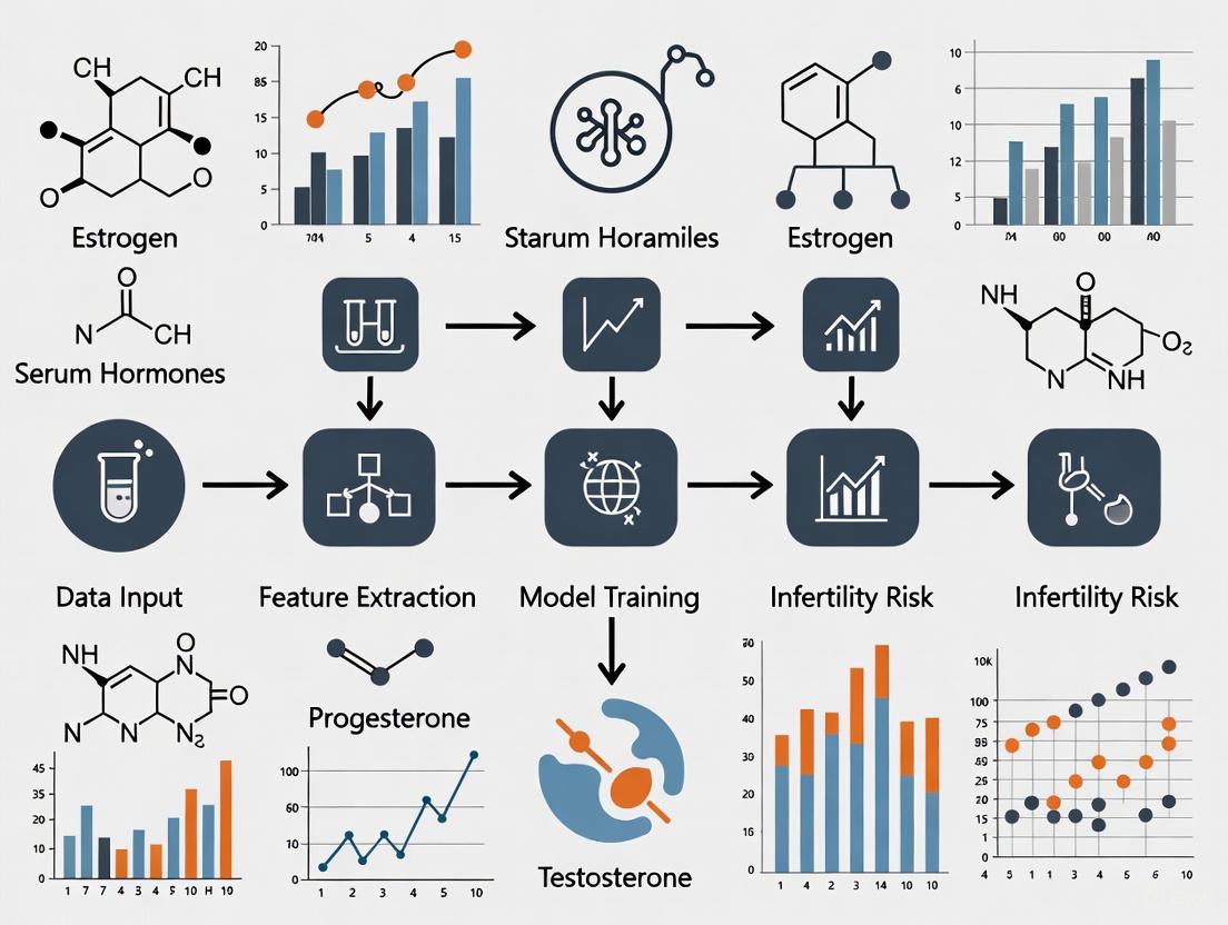
Figure 2: Machine Learning Workflow for HPG-Based Infertility Prediction. The pipeline illustrates the sequential process from data collection through clinical application, with blue nodes representing input data and computational elements.
The Scientist's Toolkit: Research Reagent Solutions
Table 3: Essential Research Reagents for HPG Axis Investigation
| Reagent/Category | Specific Examples | Research Application | Technical Notes |
|---|---|---|---|
| GnRH Agonists/Antagonists | Leuprolide, Cetrorelix, Ganirelix | Manipulation of HPG axis; studying pulsatile vs continuous GnRH effects | Continuous administration causes receptor desensitization; used in prostate cancer treatment [3] |
| Hormone Immunoassays | ELISA, CLIA, EIA kits for LH, FSH, testosterone, estradiol | Quantifying hormone levels in serum/plasma; assessing feedback mechanisms | AMH assays lack international standardization; interpret with caution [8] |
| Cell Culture Models | LβT2 gonadotrope cells, αT3-1 cells | Studying gonadotropin synthesis and regulation | LβT2 cells express both LHβ and FSHβ; useful for studying gonadotropin gene regulation [2] |
| Kisspeptin Analogues | Kisspeptin-10, Kisspeptin-54 | Probing GnRH regulation mechanisms; potential therapeutic applications | Different effects based on administration route and pattern (bolus vs continuous) [2] |
| Signal Transduction Inhibitors | PKC inhibitors, MAPK pathway inhibitors, calcium chelators | Elucidating intracellular signaling pathways in gonadotrope cells | GnRH activates multiple MAPKs (ERK1/2, JNK, p38) forming complex regulatory networks [2] [1] |
| Gene Expression Tools | Egr-1 reporters, SF-1 binding assays, chromatin immunoprecipitation | Studying gonadotropin gene regulation and epigenetic mechanisms | LHβ promoter contains conserved Egr-1 and SF-1 binding sites critical for GnRH responsiveness [2] |
The HPG axis represents a sophisticated neuroendocrine system that integrates neural, hormonal, and metabolic signals to regulate reproductive function. Understanding its complex regulatory mechanisms provides the foundation for developing advanced diagnostic and therapeutic approaches for infertility. The emergence of machine learning methods that leverage HPG axis hormone data offers promising avenues for non-invasive infertility risk assessment, particularly in male patients where FSH, LH, and testosterone-to-estradiol ratio demonstrate strong predictive value.
Future research directions should focus on:
- Multi-omics integration combining HPG axis hormones with genetic, epigenetic, and proteomic biomarkers
- Dynamic testing protocols that capture HPG axis responsiveness to stimulation challenges rather than just baseline levels
- Standardized assay platforms to enable direct comparison of hormone measurements across studies and populations
- Longitudinal studies tracking HPG axis function and fertility outcomes across the reproductive lifespan
- Interventional trials testing whether ML-guided early identification of at-risk individuals improves reproductive outcomes through timely intervention
As machine learning algorithms continue to evolve and datasets expand, HPG axis profiling is poised to become an increasingly powerful tool for personalized fertility assessment and management, ultimately improving care for individuals and couples facing reproductive challenges.
The quantitative analysis of serum hormones represents a cornerstone of diagnostic endocrinology. Within the specific field of human reproduction, the hormones Follicle-Stimulating Hormone (FSH), Luteinizing Hormone (LH), Testosterone, Estradiol, and Prolactin have established roles in regulating physiological function. The contemporary research landscape is now defined by a paradigm shift: the use of these classic biomarkers as features for machine learning (ML) models predicting clinical outcomes. This application note details the precise experimental protocols and analytical frameworks required to generate high-quality data for such research, with a specific focus on developing ML models for assessing infertility risk. The reproducibility and clinical validity of these models are fundamentally dependent on standardized data acquisition, a principle central to the methodologies described herein.
Hormonal Biomarkers: Reference Ranges and Clinical Significance
A precise understanding of hormonal reference ranges and their clinical correlations is essential for both interpreting individual patient status and for crafting meaningful predictive features for ML models. The following tables summarize key quantitative data and functional significance for the central hormonal biomarkers.
Table 1: Key Hormonal Biomarkers in Male Reproductive Endocrinology
| Hormone | Primary Function | Clinical Significance in Infertility | Key Quantitative Findings |
|---|---|---|---|
| FSH | Stimulates Sertoli cells and spermatogenesis [4] | Often elevated in spermatogenic dysfunction; clear top feature in AI infertility prediction models [4] [6] | Mean in infertile cohort: 8.845 mIU/mL (95% CI: 8.535–9.155) [4] |
| LH | Stimulates Leydig cells to produce Testosterone [4] | Elevated with low T indicates primary hypogonadism; ranked 3rd in AI feature importance [4] [9] | Mean in infertile cohort: 5.681 mIU/mL (95% CI: 5.545–5.817) [4] |
| Testosterone | Essential for libido, erectile function, and spermatogenesis [9] [10] | Low levels associated with reduced libido and ED; but not always correlated with ED in eugonadal men [9] [10] | Mean in infertile cohort: 4.741 ng/mL (95% CI: 4.672–4.810) [4] |
| Estradiol | Maintains bone density, modulates libido [9] | Imbalances can disrupt erectile function; significant independent association with ED in men without hypoandrogenism [9] [10] | Mean in infertile cohort: 26.166 pg/mL (95% CI: 25.802–26.530) [4] |
| Prolactin | Modulates dopaminergic pathways for sexual desire [9] | Hyperprolactinemia can cause hypogonadism; very low levels may also contribute to ED [9] | Mean in infertile cohort: 10.540 ng/mL (95% CI: 9.865–11.214) [4] |
Table 2: Hormonal Associations with Clinical Conditions Beyond Infertility
| Condition | Relevant Hormones | Key Associations and Findings |
|---|---|---|
| Erectile Dysfunction (ED) | Testosterone, Free Testosterone, DHEA-S, Estradiol, SHBG | Total and Free Testosterone levels progressively decrease with ED severity. Free Testosterone is a more sensitive marker, with median levels below the normal threshold in all ED groups [9]. |
| Gender-Affirming Hormone Therapy (GAHT) | Testosterone, Estradiol, Prolactin | GAHT is associated with QTc interval prolongation in transgender women and shortening in transgender men, corresponding to the restoration of sexual dimorphism observed in cisgender adults [11]. |
| Polycystic Ovary Syndrome (PCOS) | Anti-Müllerian Hormone (AMH), LH, Testosterone | AMH has emerged as a key biomarker reflecting ovarian reserve and may play a role in pathogenesis. PCOS is now considered a cardiovascular disease risk-enhancing factor [12]. |
| Turner Syndrome | Anti-Müllerian Hormone (AMH) | AMH is a reliable biomarker for ovarian reserve and prediction of spontaneous puberty, with significantly lower levels in TS patients versus controls (WMD: -3.04 ng/mL) [13]. |
Experimental Protocols for Hormone Assay and Data Collection
Standardized Pre-Analytical Protocol for Blood Sample Collection
Robust ML models require datasets generated from standardized laboratory practices to minimize technical noise.
- Patient Preparation: Participants should provide samples after an 8–10 hour fast. For male infertility studies, a defined period of sexual abstinence (e.g., 2-5 days) may be recommended prior to semen analysis [4].
- Sample Timing: Blood collection must be performed in the morning (e.g., before 10:00 AM) to account for diurnal variation in hormone levels, particularly for testosterone [9] [10].
- Sample Processing: Collect venous blood into serum separator tubes (e.g., BD Vacutainer). After collection, allow samples to clot for 30 minutes at room temperature. Subsequently, centrifuge to isolate serum, aliquot into sterile tubes (e.g., Eppendorf), and store at -80°C until analysis to prevent degradation [9].
Analytical Protocol for Hormone Quantification
The choice of assay methodology significantly impacts result accuracy and inter-study comparability.
- Recommended Platform: Utilize automated chemiluminescence immunoassay (CLIA) systems, such as the ARCHITECT i1000 or i2000 series (Abbott Diagnostics) or similar platforms from Roche Diagnostics [11] [9]. These systems provide the high throughput and precision required for large-scale studies.
- Methodology Specifics:
- For the majority of hormones (FSH, LH, Prolactin, Estradiol), standard CLIA methods are sufficient and widely used [9] [10].
- For Total Testosterone, liquid chromatography–mass spectrometry (LC-MS/MS) is considered the gold standard due to its high specificity and accuracy, especially at lower concentrations [11].
- Quality Control: Each assay run must include internal quality controls at low, medium, and high concentrations. Participation in external quality assurance (proficiency testing) programs is mandatory for laboratory accreditation.
Clinical Phenotyping Protocol for Model Ground Truth
The predictive power of an ML model is contingent on the accuracy of its diagnostic labels.
- For Male Infertility Studies: The ground truth for model training must be established via standard semen analysis conducted according to the latest World Health Organization (WHO) laboratory manual [4] [6]. Key parameters include:
- Sperm Concentration: Azoospermia, cryptozoospermia, oligozoospermia.
- Sperm Motility: Asthenozoospermia.
- Total Motile Sperm Count (TMSC): Often used as a key outcome threshold (e.g., 9.408 × 10^6 defined as lower limit of normal) [4].
- For Erectile Dysfunction Studies: Patient assessment should be conducted using the validated International Index of Erectile Function (IIEF-15 or IIEF-5) questionnaire to provide a quantitative and standardized measure of dysfunction severity [9] [10].
The Hypothalamic-Pituitary-Gonadal (HPG) Axis: A Systems View
The hormonal biomarkers detailed in this document do not function in isolation but are components of an integrated endocrine system. The following diagram illustrates the core feedback loops of the HPG axis, the primary system governing reproductive function. A systems-level understanding of these interactions is critical for generating meaningful features for machine learning models, as it reveals potential synergies and regulatory relationships between biomarkers.
Machine Learning Workflow for Infertility Risk Prediction
Translating standardized hormone data into a predictive ML model requires a structured pipeline from data pre-processing to model deployment. The following diagram outlines this workflow, highlighting the critical steps that ensure the developed model is robust, accurate, and clinically actionable.
Protocol for Model Development and Validation
The workflow illustrated above depends on rigorous execution at each stage.
- Data Pre-processing: Address missing values appropriately (e.g., imputation or removal). Apply Z-score normalization to scale numerical hormone data, preventing features with larger intrinsic scales from dominating the model [5].
- Feature Engineering: Beyond raw hormone levels, create derived ratios that have biological plausibility. The Testosterone-to-Estradiol (T/E2) ratio has been identified as the second most important predictive feature after FSH in several models [4].
- Model and Algorithm Selection: Implement and compare multiple supervised learning algorithms to identify the best performer for your dataset. High-performing algorithms in this domain include:
- Model Validation: Employ 10-fold cross-validation to assess model generalizability and avoid overfitting. Evaluate performance using Area Under the Curve (AUC) for Receiver Operating Characteristic (ROC) and Precision-Recall (PR) curves. The model by Kobayashi et al. achieved an AUC of 74.42% [4] [6].
The Scientist's Toolkit: Essential Research Reagents and Materials
Table 3: Essential Reagents and Materials for Hormone and ML Research
| Item | Specification/Example | Critical Function |
|---|---|---|
| Automated Immunoassay System | ARCHITECT i1000/i2000SR (Abbott), Cobas e801 (Roche) | High-throughput, precise quantification of FSH, LH, Prolactin, Estradiol via chemiluminescence (CLIA) [9]. |
| LC-MS/MS System | Agilent 6470, Sciex Triple Quad 6500+ | Gold-standard quantification for testosterone and other steroids, providing superior specificity and accuracy [11]. |
| Blood Collection System | BD Vacutainer (Serum Separator Tubes with clot activator) | Standardized sample collection and serum separation for consistent pre-analytical conditions [9]. |
| Laboratory Software | CalECG, Version 3.7 (AMPS LLC) | For semi-automatic analysis of complex physiological data (e.g., ECG), demonstrating the principle of using specialized software for feature extraction [11]. |
| AI Development Platform | No-code AI software (e.g., Prediction One, AutoML Tables) | Allows researchers without deep coding expertise to build and compare initial predictive models from structured data [4]. |
| Statistical & Coding Environment | R Programming Language (with packages: caret, SuperLearner, e1071, rpart) |
Provides a flexible, open-source environment for data pre-processing, machine learning, and statistical validation [5]. |
The diagnosis and treatment of infertility rely heavily on the precise correlation between serum hormone levels and direct measures of reproductive function: semen analysis in men and ovarian reserve in women. Hormonal dysregulation of the hypothalamic-pituitary-gonadal (HPG) axis serves as a critical indicator of underlying pathology and treatment response. This document synthesizes recent clinical evidence and establishes standardized protocols for investigating these correlations, providing a foundational context for the development of machine learning models that predict infertility risk from serum biomarkers. The integration of quantitative hormone data with clinical outcomes enables more precise, individualized treatment strategies and enhances the predictive capability of computational tools.
Quantitative Data Synthesis
Key Hormonal Correlates in Male Infertility
Table 1: Hormonal Profiles and Predictive Values for Male Infertility Conditions
| Condition | FSH (mIU/mL) | LH (mIU/mL) | Testosterone (ng/mL) | T/E2 Ratio | Predictive Accuracy |
|---|---|---|---|---|---|
| Normal Fertility [4] | 8.85 (CI: 8.54-9.16) | 5.68 (CI: 5.55-5.82) | 4.74 (CI: 4.67-4.81) | 19.92 (CI: 19.54-20.29) | - |
| Non-Obstructive Azoospermia (NOA) [4] [6] [14] | Significantly Elevated | Variable | Variable | Significant Reduction | 100% (AI Model Prediction) [14] |
| Oligo/Asthenozoospermia [4] | Elevated | Variable | Variable | Reduced | - |
| AI Model Feature Importance [4] | 1st (92.24%) | 3rd (1.81%) | 4th/5th | 2nd (3.37%) | AUC: 74.2-74.4% [4] |
Key Hormonal Correlates in Female Infertility and Ovarian Reserve
Table 2: Hormonal and Ultrasonographic Predictors of Ovarian Response in IVF
| Parameter | Role in Ovarian Reserve Assessment | Correlation with Gn Starting Dose | Predictive Value in POI |
|---|---|---|---|
| AMH [15] [16] | Reflects pool of early antral follicles; cycle-stable [15] | Significant negative correlation (P<0.05) [16] | Superior predictor of follicular growth (AUC: 0.957); optimal threshold: 2.45 pg/mL [15] |
| Basal FSH (bFSH) [15] [16] | Indirect measure of follicular pool; high levels indicate diminished reserve | Significant positive correlation (P<0.05) [16] | Shorter amenorrhea duration and lower levels in POI patients with follicular development [15] |
| Antral Follicle Count (AFC) [16] | Direct ultrasonographic count of recruitable follicles | Significant negative correlation (P<0.05) [16] | - |
| Age [16] | Non-hormonal factor influencing oocyte quantity and quality | Significant positive correlation (P<0.05) [16] | - |
| BMI [16] | Modifies metabolic and endocrine environment | Significant positive correlation (P<0.05) [16] | - |
Experimental Protocols
Protocol for Investigating Male Infertility Using Serum Hormones and AI Modeling
Objective: To develop a machine learning model for predicting male infertility risk based solely on serum hormone levels, bypassing initial semen analysis [4] [6].
Patient Population and Data Collection:
- Cohort: 3,662 patients undergoing fertility evaluation (2011-2020) [4].
- Inclusion: Patients with complete semen analysis and serum hormone profiles.
- Data Extracted: Age, LH, FSH, Prolactin (PRL), Testosterone, Estradiol (E2), and calculated T/E2 ratio [4].
- Outcome Variable: Total motile sperm count (TMSC), with a value below 9.408 x 10^6 defined as abnormal [4] [14].
Machine Learning Methodology:
- Software & Algorithms: Utilize no-code AI platforms (e.g., Prediction One) or code-based libraries (e.g.,
caretin R). Apply algorithms such as Support Vector Machines (SVM) and ensemble methods (e.g., SuperLearner) [4] [5]. - Model Training & Validation: Split data into training (e.g., 80%) and validation (e.g., 20%) sets. Use 10-fold cross-validation to assess model performance and prevent overfitting [5].
- Performance Metrics: Evaluate using Area Under the Curve (AUC) of the Receiver Operating Characteristic (ROC) curve, accuracy, precision, and recall [4] [5]. Analyze feature importance to identify key hormonal predictors [4].
Protocol for Correlating AMH with Follicular Growth in Primary Ovarian Insufficiency (POI)
Objective: To evaluate the efficacy of a highly sensitive AMH assay in predicting follicular development during prolonged controlled ovarian stimulation (COS) in POI patients [15].
Patient Selection and Design:
- Design: Retrospective cohort study.
- Patients: 165 POI patients undergoing 504 long COS cycles [15].
- Inclusion Criteria: Age 20-48, last menstruation before 40, serum FSH >25 mIU/mL and E2 <20 pg/mL on two occasions, >3 months amenorrhea without hormone therapy [15].
- Stimulation Protocol: Use of GnRH-agonist (Buserelin acetate) for pituitary down-regulation, followed by stimulation with human menopausal gonadotrophin or recombinant FSH for over four weeks [15].
Measurement and Analysis:
- AMH Measurement: Serum AMH levels measured at 3 weeks (days 18-27) post-stimulation initiation using the highly sensitive pico AMH ELISA (MenoCheck pico AMH, Ansh Labs) with a LoD of 1.3 pg/mL [15].
- Primary Outcome: Follicular development defined by ultrasonically detectable antral follicles (≥2 mm) [15].
- Statistical Analysis: ROC curve analysis to determine the predictive power and optimal threshold of 3-week AMH levels for follicular growth. Correlation analysis (e.g., Pearson's R) between AMH levels and time to follicular detection [15].
Protocol for Individualizing Gonadotropin Starting Dose in Normal Ovarian Responders
Objective: To create and validate a clinical prediction model (nomogram) for determining the optimal Gn starting dose in NOR patients undergoing their first IVF/ICSI-ET cycle [16].
Study Population and Design:
- Design: Retrospective analysis of 535 first IVF/ICSI-ET cycles.
- Inclusion: NOR patients (aged 20-38) with 5-15 oocytes retrieved, undergoing GnRH-agonist or antagonist protocols [16].
- Exclusion: Patients with PCOS, endocrine, metabolic, or autoimmune diseases [16].
Data Collection and Model Development:
- Predictor Variables: Collect age, BMI, basal FSH (bFSH), AMH, and AFC on cycle day 2-3 [16].
- Outcome Variable: The actual Gn starting dose (IU) used in the cycle [16].
- Statistical Analysis:
- Randomly split data into training (60%) and validation (40%) sets.
- Perform univariate and multivariate linear regression to identify factors significantly (P<0.05) associated with the Gn dose.
- Construct a nomogram based on the significant predictors.
- Validate the model by comparing the predicted dose to the actual dose in the validation set, using metrics like Mean Absolute Error (MAE) and a t-test (P>0.05 indicates no significant difference) [16].
Signaling Pathways and Physiological Correlations
The Hypothalamic-Pituitary-Gonadal (HPG) Axis
The HPG axis is the central regulatory system for reproduction, and its dysregulation is a primary source of infertility [17]. Understanding this pathway is fundamental to interpreting hormone profiles.
The Scientist's Toolkit: Research Reagent Solutions
Table 3: Essential Reagents and Assays for Hormonal and Functional Analysis in Infertility Research
| Item Name | Manufacturer (Example) | Function & Application |
|---|---|---|
| Pico AMH ELISA | Ansh Labs (MenoCheck pico AMH) [15] | Highly sensitive quantification of very low AMH levels (LoD: 1.3 pg/mL); crucial for assessing patients with severely diminished ovarian reserve, such as POI. |
| Automated Immunoassay Analyzer | TOSOH (AIA-900) [15] | Automated, high-throughput measurement of reproductive hormones (FSH, LH, E2, P, PRL) in serum samples. |
| Access AMH Immunoassay / Gen II AMH ELISA | Beckman Coulter [15] | Standard clinical assays for measuring AMH levels in patients with normal to moderately reduced ovarian reserve. |
| Recombinant FSH / Human Menopausal Gonadotrophin (hMG) | Various | Used in Controlled Ovarian Stimulation (COS) protocols to induce multifollicular development for IVF [15] [16]. |
| GnRH Agonist (e.g., Buserelin acetate) | Various | Used for pituitary down-regulation in long-protocol IVF cycles to prevent premature luteinizing hormone surge [15] [16]. |
| GnRH Antagonist | Various | Used in flexible IVF protocols to prevent premature LH surge by competitively blocking GnRH receptors [16]. |
| Vitrification Kit | Kitazato Corp. (Cryotop) [15] | For the cryopreservation of oocytes and embryos post-retrieval, utilizing ultra-rapid cooling to maintain cellular viability. |
| No-Code AI Creation Software | Prediction One, AutoML Tables [4] [6] | Enables researchers without advanced programming skills to develop and validate predictive machine learning models using clinical data. |
Infertility, defined as the failure to conceive after 12 months of regular unprotected intercourse, affects approximately 15% of couples worldwide [18]. Traditional diagnostic approaches have relied heavily on isolated hormone measurements, including follicle-stimulating hormone (FSH), luteinizing hormone (LH), anti-Müllerian hormone (AMH), and prolactin, to assess reproductive function [19]. These biomarkers are typically interpreted individually using population-based reference ranges, despite compelling evidence that their predictive value is limited when examined in isolation [20]. The complex, multifactorial nature of infertility necessitates a more sophisticated analytical approach that can integrate hormonal data with demographic, clinical, and lifestyle factors to provide clinically meaningful prognostic information.
The fundamental limitation of single-hormone testing lies in its reductionist approach to a systems biology challenge. Female reproductive function involves intricate feedback mechanisms between the hypothalamic-pituitary-ovarian axis, where hormones interact in dynamic, non-linear patterns throughout the menstrual cycle [20]. Isolated measurements capture merely a static snapshot of this complex, fluctuating system, failing to represent the integrated hormonal milieu that ultimately determines reproductive outcomes. Furthermore, hormone concentrations exhibit significant variation across different female hormonal statuses—including oral contraceptive pill users, menstrual cycle phases, and menopausal status—further complicating the interpretation of single measurements without proper contextualization [20].
Quantitative Evidence: The Limitations of Single-Marker Approaches
Robust scientific evidence demonstrates the inherent limitations of isolated hormone testing for infertility assessment. A comprehensive analysis of 171 serum biomarkers revealed that 68% (117 analytes) showed significant variation with sex and female hormonal status, indicating that single hormone measurements without proper contextualization can be highly misleading [20]. This biological variability directly impacts clinical test reproducibility and diagnostic accuracy, contributing to the poor translational success of biomarker studies from research to clinical practice.
Table 1: Impact of Biological Variability on Serum Biomarker Levels
| Variability Factor | Number of Affected Biomarkers | False Discovery Rate in Unmatched Studies | Key Clinical Implications |
|---|---|---|---|
| Sex differences | 96 biomarkers | Up to 39.6% | Male and female reference ranges required for accurate interpretation |
| Oral contraceptive use | 55 biomarkers | Up to 41.4% | Contraceptive status must be recorded and matched in study designs |
| Menopausal status | 26 biomarkers | Not quantified | Age and menopausal status critically impact reference values |
| Menstrual cycle phase | 5 biomarkers | Not quantified | Timing within cycle essential for proper interpretation |
The clinical consequences of these limitations are substantial. Simulation studies demonstrate that when patient and control groups are not matched for sex, researchers can encounter false positive findings in nearly 40% of measured analytes [20]. Similarly, when premenopausal female groups differ in oral contraceptive usage, false discoveries can affect over 41% of biomarkers. These staggering rates of misinterpretation highlight the critical inadequacy of single-marker approaches that fail to account for fundamental biological variabilities.
Beyond the statistical challenges, isolated hormone testing provides insufficient prognostic value for clinical decision-making. A retrospective study of 1,931 patients showed that no single hormone parameter alone could accurately predict clinical pregnancy rates in either IVF/ICSI or IUI treatments [21]. The random forest model, which integrated multiple hormonal, demographic, and treatment parameters, demonstrated superior performance with accuracy exceeding standalone hormone assessments, underscoring the limitation of reductionist approaches [21].
Machine Learning Solutions for Infertility Risk Assessment
Machine learning (ML) approaches represent a paradigm shift in infertility assessment by simultaneously analyzing multiple hormonal, demographic, and clinical parameters to generate integrated risk predictions. These models capture complex, non-linear relationships between variables that conventional statistical methods often miss, providing superior prognostic accuracy [19]. The HyNetReg model exemplifies this approach, combining deep feature extraction using neural networks with regularized logistic regression to achieve enhanced predictive performance for infertility outcomes based on hormonal and demographic profiles [19].
Table 2: Performance Comparison of Predictive Modeling Approaches
| Model Type | Key Features | Accuracy Metrics | Advantages | Limitations |
|---|---|---|---|---|
| Isolated hormone testing | Single hormone interpretation | Varies by hormone | Simple to implement, low cost | Poor prognostic value, high false discovery rates |
| Traditional statistical models | Multivariable regression | Not consistently reported | Familiar methodology, interpretable | Limited capture of complex interactions |
| Random forest | Ensemble decision trees | Highest accuracy in comparative studies [21] | Handles non-linear relationships, robust to outliers | Less interpretable than simpler models |
| HyNetReg hybrid model | Neural network feature extraction + logistic regression | Superior to traditional logistic regression [19] | Captures complex patterns, improved classification | Computationally intensive |
| Machine learning center-specific (MLCS) | Center-specific training and validation | Improved minimization of false positives/negatives vs. SART model [22] | Adapts to local patient populations, clinically relevant | Requires substantial center-specific data |
The clinical utility of ML approaches extends beyond basic infertility prediction to specific treatment applications. For fresh embryo transfer in patients with endometriosis, an XGBoost model incorporating eight key predictors—including AMH, female age, antral follicle count, infertility duration, and GnRH agonist protocol—demonstrated superior predictive performance for live birth outcomes compared to seven other machine learning models [23]. The model achieved an AUC of 0.852 in the test set, significantly outperforming traditional approaches and enabling more personalized treatment recommendations for this challenging patient population [23].
The implementation of ML models in clinical settings has demonstrated tangible improvements in treatment outcomes. An AI model trained on 53,000 IVF cycles and designed to optimize trigger timing resulted in significantly improved oocyte yield when clinicians followed the model's recommendations compared to physician estimates alone [24]. Cycles aligned with AI-guided trigger timing yielded an average of 3.8 more mature oocytes and 1.1 more usable embryos, highlighting the clinical impact of data-driven decision support systems [24].
Experimental Protocols for Predictive Model Development
Data Collection and Preprocessing Methodology
Comprehensive data collection forms the foundation of robust predictive models for infertility risk assessment. The following protocol outlines standardized procedures for acquiring and preparing data for model development:
Patient Population and Inclusion Criteria: Recruit patients presenting for infertility evaluation and treatment. Inclusion criteria should encompass complete demographic data, hormonal profiles, and treatment outcomes. Standard exclusion criteria typically include use of donor gametes, surrogacy arrangements, and cycles with incomplete data (>50% missing values) [21].
Hormonal Assessment Protocol: Collect blood samples during the early follicular phase (day 2-4) of the menstrual cycle for basal hormone measurements. Process samples within 2 hours of collection and store at -80°C until analysis. Analyze reproductive hormones using standardized immunoassay platforms (e.g., Beckman Coulter DxI 800 Immunoassay Analyzer) with consistent quality control procedures [25]. Essential hormones include FSH, LH, AMH, estradiol (E2), and prolactin.
Clinical and Demographic Data Collection: Record comprehensive patient characteristics including female age, male age, body mass index (BMI), infertility duration and type (primary/secondary), ovarian reserve markers (antral follicle count), and semen analysis parameters according to WHO guidelines [25].
Data Preprocessing Pipeline: Implement a multi-step preprocessing protocol:
- Missing Data Imputation: Apply sophisticated imputation methods such as Multi-Level Perceptron (MLP) to predict missing values, which provides superior results compared to traditional mean imputation [21].
- Data Normalization: Use standard scaling or normalization techniques to address varying measurement scales across different biomarkers.
- Class Imbalance Handling: Apply Synthetic Minority Over-sampling Technique (SMOTE) to address class imbalance in the dataset, particularly when modeling relatively rare outcomes such as clinical pregnancy or live birth [25].
Model Development and Validation Framework
The development of robust, clinically applicable predictive models requires a structured approach to model selection, training, and validation:
Predictor Variable Selection: Employ feature selection algorithms such as Least Absolute Shrinkage and Selection Operator (LASSO) and Recursive Feature Elimination (RFE) to identify the most informative predictors for model inclusion [23]. For infertility applications, key predictors typically include female age, AMH, FSH, infertility duration, and specific treatment parameters.
Model Architecture and Training: Implement multiple machine learning algorithms to compare performance, including random forest, XGBoost, logistic regression, support vector machines, and artificial neural networks [21] [23]. Utilize a nested cross-validation framework with outer validation using stratified 5-fold cross-validation for training/testing splits and inner 5-fold stratified cross-validation for hyperparameter optimization [25].
Model Validation Protocol: Implement comprehensive validation procedures:
- Internal Validation: Use k-fold cross-validation (typically k=10) to evaluate model performance and avoid overfitting, particularly important for smaller datasets [21].
- External Validation: Reserve a portion of the dataset (typically 20-30%) that is not used in model development for final performance assessment [21] [23].
- Live Model Validation (LMV): Test model performance on out-of-time test sets comprising patients who received treatment contemporaneous with clinical model usage to assess ongoing applicability and detect data drift [22].
Performance Metrics and Clinical Utility Assessment: Evaluate models using multiple metrics including area under the receiver operating characteristic curve (ROC-AUC), precision-recall AUC (PR-AUC), F1 score, Brier score, and calibration curves [23] [22]. Supplement statistical evaluation with decision curve analysis to assess clinical utility across different probability thresholds [23] [25].
The Scientist's Toolkit: Essential Research Reagents and Analytical Platforms
Table 3: Essential Research Reagents and Platforms for Hormonal Predictive Modeling
| Reagent/Platform | Specific Function | Application Context | Technical Considerations |
|---|---|---|---|
| Multiplex Immunoassay Platforms (e.g., Human DiscoveryMAP) | Simultaneous measurement of 171+ proteins and small molecules | Comprehensive biomarker profiling for model development [20] | Enables broad biomarker discovery but requires validation of individual assays |
| Chemiluminescence Immunoassay Analyzer (e.g., Beckman Coulter DxI 800) | Quantitative measurement of reproductive hormones | Standardized AMH, FSH, LH, E2 assessment in clinical samples [25] | Provides clinical-grade accuracy essential for valid model inputs |
| Leica Biosystems Aperio AT2 Digital Pathology Scanner | Digitization of H&E-stained histopathology slides at 20x magnification | Digital pathology feature extraction for multimodal AI models [26] | Enables integration of histopathological features with clinical data |
| Isolate Double-Density Gradient Centrifugation Media | Sperm selection and preparation for ART procedures | Standardized semen processing for consistent parameter assessment [25] | Critical for obtaining reproducible male factor parameters |
| Sperm Chromatin Structure Assay (SCSA) Reagents | Assessment of sperm DNA fragmentation index (DFI) | Evaluation of sperm quality parameter predictive of fertilization success [25] | Standardized protocol essential for comparable results across studies |
| Resnet-50 Feature Extraction Model | Self-supervised learning for digital pathology image analysis | Extraction of meaningful features from histopathology images without manual annotation [26] | Requires substantial computational resources for training and implementation |
The limitations of isolated hormone testing in infertility assessment are both significant and well-documented. Single hormone measurements fail to capture the complex, dynamic interactions of the endocrine system and exhibit substantial biological variability that compromises their diagnostic and prognostic utility. Machine learning approaches that integrate multiple hormonal parameters with clinical, demographic, and treatment factors represent a transformative advancement in infertility risk assessment. These models demonstrate superior performance compared to both traditional isolated hormone testing and conventional statistical approaches, providing more accurate prognostic information to guide clinical decision-making.
The implementation of standardized protocols for data collection, preprocessing, and model validation is essential for developing robust, clinically applicable predictive tools. As the field progresses toward a systems medicine approach to infertility care, integrating multi-omics data and leveraging advanced analytical techniques will further enhance our ability to provide personalized, predictive, and preventive reproductive healthcare. The era of data-driven medicine in infertility has arrived, offering new hope for the millions of couples struggling with infertility worldwide.
Building the Model: Data, Algorithms, and Feature Engineering for Hormonal Data
Within the research domain of developing machine learning (ML) models for predicting infertility risk from serum hormones, the integrity of the underlying data is paramount. This document outlines critical application notes and protocols for data sourcing and preprocessing, with a specific focus on handling missing values and defining patient cohorts. These steps are foundational to building robust, accurate, and reliable predictive models. Proper execution ensures that the model's findings on the relationship between hormone levels (e.g., FSH, LH, Testosterone) and infertility outcomes are valid and clinically meaningful [4].
Handling Missing Data in Hormonal Datasets
Missing data is a common occurrence in medical datasets and, if not handled appropriately, can introduce significant bias, reduce statistical power, and lead to incorrect conclusions [27]. The approach to handling missing values must be deliberate and justified.
Types and Identification of Missing Values
Understanding why data is missing is crucial for selecting the correct handling strategy. The underlying mechanism is typically categorized as follows:
- Missing Completely at Random (MCAR): The probability of data being missing is unrelated to any observed or unobserved variables. For example, a data point is missing due to a random processing error.
- Missing at Random (MAR): The probability of missingness depends on other observed variables but not on the missing value itself. For instance, the missingness of a specific hormone value might be related to the patient's age group, which is fully recorded.
- Missing Not at Random (MNAR): The probability of missingness is related to the unobserved missing value itself. An example would if individuals with very high or very low hormone levels are less likely to report them [27] [28].
The first step is to identify missing values, which can be represented as NaN, NULL, None, or other placeholders like -999 [27] [28]. In Python, using the pandas library is standard practice:
Strategies and Protocols for Handling Missing Values
The choice of strategy depends on the proportion of missing data, its mechanism, and the specific analytical goals. The following table summarizes the primary methods.
Table 1: Strategies for Handling Missing Values in Hormonal Data
| Strategy | Description | Best Use Case | Pros & Cons |
|---|---|---|---|
| Listwise Deletion | Removing any row (participant) that has a missing value in any of the variables used in the analysis. | Data is MCAR and the number of deleted rows is small (<5% of the dataset). | Pros: Simple, quick. Cons: Can reduce sample size significantly and introduce bias if data is not MCAR [27] [28]. |
| Mean/Median/Mode Imputation | Replacing missing values with the mean (for normally distributed data), median (for skewed data), or mode (for categorical data) of the available cases in that column. | MCAR data; numerical variables where a simple, fast fix is needed for a small number of missing values. | Pros: Easy and fast to implement. Cons: Can distort the data distribution and underestimate variance [27] [29]. |
| Forward Fill/ Backward Fill | Filling missing values with the last (forward fill) or next (backward fill) valid observation in the dataset. | Time-series data or data where the order of records is meaningful. | Pros: Preserves the order of data points. Cons: Can be inaccurate if the adjacent values are not similar [27]. |
| Interpolation | Estimating missing values based on other data points, often using methods like linear or polynomial interpolation to capture trends. | Data with a discernible trend, such as hormone levels measured over time. | Pros: More accurate than simple imputation as it captures trends. Cons: Assumes a specific pattern (e.g., linear) between points [27] [29]. |
| K-Nearest Neighbors (KNN) Imputation | Replacing a missing value with the mean or median of the 'k' most similar participants (neighbors) based on other available variables. | MAR data; datasets with multiple correlated variables. | Pros: Can be more accurate than simple imputation by using information from similar cases. Cons: Computationally intensive for large datasets [28]. |
| Model-Based Imputation | Using a predictive model (e.g., regression, Random Forest) to estimate missing values based on all other available variables. | MAR data; complex datasets where other variables are strong predictors of the missing one. | Pros: Potentially the most accurate method. Cons: Complex to implement; risk of overfitting [29]. |
Recommended Protocol for Hormonal Data: For a dataset of serum hormone levels (FSH, LH, Testosterone, etc.) aimed at training an ML model, the following workflow is recommended.
Cohort Definition for Infertility Risk Studies
A cohort study is an observational research design that follows a group of people (a cohort) over a period of time to investigate how specific factors affect the incidence of an outcome [30] [31]. In the context of infertility risk, this design is powerful for establishing temporality—confirming that exposure (serum hormone levels) was measured before the outcome (infertility diagnosis) was determined.
Cohort Study Design and Selection
The two primary types of cohort studies are prospective and retrospective, both applicable to infertility research.
Table 2: Types of Cohort Studies for Infertility Research
| Cohort Type | Description | Application in Infertility Risk | Advantages & Disadvantages |
|---|---|---|---|
| Prospective Cohort | A group of participants without the outcome of interest is recruited and followed forward in time to see who develops the outcome. | Recruiting men with no current infertility diagnosis, measuring their baseline serum hormones, and following them for several years to see who later receives an infertility diagnosis. | Advantages: High data quality control, clear temporality. Disadvantages: Time-consuming and expensive [30] [31]. |
| Retrospective Cohort | Researchers look back at historical data to identify a cohort based on past exposure status and then determine if they have since developed the outcome. | Using existing medical records to identify men whose serum hormones were measured 5 years ago, and then reviewing their subsequent fertility status up to the present. | Advantages: Faster and less costly than prospective studies. Disadvantages: Reliance on pre-existing data of potentially variable quality [30] [31]. |
Key Considerations for Cohort Definition:
- Inclusion/Exclusion Criteria: Clearly define the cohort's characteristics. For example: "The cohort will include males aged 20-45 who presented for fertility evaluation, with complete baseline serum hormone profiles (FSH, LH, Testosterone). Exclusion criteria: history of vasectomy, obstructive azoospermia, or hormonal treatment within the last 6 months." [30]
- Exposure and Outcome Measurement:
- Exposure: Precisely define the serum hormone measures (e.g., "baseline FSH level in mIU/mL").
- Outcome: Clearly define the infertility outcome based on standardized criteria, such as the WHO semen analysis guidelines [4] or clinical diagnosis.
- Minimizing Bias: Be aware of biases like attrition bias (participants dropping out in a prospective study) and information bias (inaccurate measurement of exposure or outcome) [31].
The following diagram illustrates the logical structure of a cohort study in this context.
Experimental Protocol: Building an ML Model for Infertility Risk
This protocol integrates the concepts of data preprocessing and cohort definition, drawing from recent research that successfully predicted male infertility risk using serum hormones and AI [4].
Study Design and Data Sourcing
- Cohort Definition: A retrospective cohort study design is employed.
- Participants: The study uses data from 3,662 male patients who underwent both semen analysis and serum hormone testing [4].
- Inclusion/Exclusion: Participants are classified based on semen analysis results (e.g., normal, oligozoospermia, azoospermia) according to WHO standards.
Data Collection and Preprocessing
- Variables Collected: The following data is extracted from medical records:
- Handling Missing Values: The specific method used in the source study is not detailed, but based on best practices (Section 2.2), a model-based imputation or KNN imputation would be appropriate for a dataset of this nature to preserve sample size and statistical power.
Model Training and Evaluation
- ML Technique: The referenced study used AI/Machine Learning models (Prediction One and AutoML Tables) [4].
- Feature Importance: The study found that FSH was the most important predictive feature, followed by T/E2 ratio and LH [4].
- Performance Metrics: The model's performance was evaluated using the Area Under the Curve (AUC) of the Receiver Operating Characteristic (ROC) curve, achieving approximately 74.4%, and other metrics like Precision and Recall [4].
The Scientist's Toolkit: Research Reagent Solutions
The following table details key materials and tools essential for research in this field.
Table 3: Essential Research Reagents and Materials for Serum Hormone-Based Infertility Studies
| Item | Function/Description | Example/Note |
|---|---|---|
| Immunoassay Kits | To quantitatively measure serum levels of specific hormones (FSH, LH, Testosterone, Estradiol, Prolactin). | Commercial ELISA (Enzyme-Linked Immunosorbent Assay) or CLIA (Chemiluminescent Immunoassay) kits are standard. |
| WHO Laboratory Manual | The international standard for the examination and processing of human semen to define infertility outcomes. | "WHO Laboratory Manual for the Examination and Processing of Human Semen" (e.g., 6th Edition, 2021) [4]. |
| Data Analysis Software | For statistical analysis, data preprocessing, and machine learning model development. | Python (with pandas, scikit-learn) or R. The cited study used "Prediction One" and "AutoML Tables" [4]. |
| Biobank Storage | For the long-term, stable storage of serum samples at ultra-low temperatures for future validation or testing. | Freezers maintaining -80°C. |
| Automated Semen Analyzer (CASA) | For objective, computer-assisted analysis of semen parameters (concentration, motility, morphology). | Provides standardized, reproducible data for defining the outcome variable. |
Within the development of machine learning (ML) models for assessing infertility risk from serum hormones, feature selection is a critical step that directly impacts model performance, interpretability, and clinical applicability. Identifying the most predictive biochemical markers allows for the creation of robust, efficient, and cost-effective diagnostic tools. This document outlines key predictive hormones and ratios, summarizes supporting quantitative evidence, and provides detailed protocols for their measurement and integration into ML workflows, contextualized within a broader thesis on computational approaches to infertility risk assessment.
Research demonstrates that a select group of serum hormones and their derived ratios serve as powerful predictors for male infertility risk. The table below summarizes the key features and their relative importance as identified in a large-scale study developing an AI model for determining male infertility risk without semen analysis [4].
Table 1: Key Predictive Hormones and Ratios for Male Infertility Risk Assessment
| Feature Name | Feature Type | Reported Feature Importance (Ranking) | Key Rationale & Association |
|---|---|---|---|
| Follicle-Stimulating Hormone (FSH) | Hormone | 1st (Highest) [4] | Primary indicator of spermatogenic function; often elevated in spermatogenic dysfunction [4]. |
| Testosterone to Estradiol Ratio (T/E2) | Calculated Ratio | 2nd [4] | Reflects androgen-estrogen balance; crucial for spermatogenesis and bone health [4] [32]. |
| Luteinizing Hormone (LH) | Hormone | 3rd [4] | Stimulates Leydig cells to produce testosterone; indicates pituitary-testicular axis function [4]. |
| Testosterone | Hormone | 4th-5th [4] | Primary androgen required, with FSH, for spermatogenesis [4] [32]. |
| Estradiol (E2) | Hormone | 6th [4] | Formed from testosterone via aromatase; has negative feedback effects [4] [32]. |
| Prolactin (PRL) | Hormone | 7th [4] | Hyperprolactinemia can suppress hypothalamic-pituitary-gonadal axis [4]. |
| Age | Demographic Variable | 4th-5th [4] | Confounding factor influencing hormonal levels and overall fertility potential [4]. |
The predictive power of these features is validated by ML model performance. A model utilizing these serum markers achieved an Area Under the Curve (AUC) of 74.42% in predicting male infertility risk, demonstrating the viability of this approach [4].
Experimental Protocols for Key Feature Assessment
Protocol: Blood Collection and Serum Hormone Profiling
This protocol details the standard procedure for obtaining the serum samples used for hormone analysis in predictive modeling.
1. Principle: To collect high-quality blood serum for the accurate quantification of reproductive hormones via immunoassay or mass spectrometry.
2. Reagents & Equipment:
- Serum separator tubes (SST)
- Venipuncture kit (tourniquet, alcohol swabs, needles, adhesive bandage)
- Centrifuge
- -20°C or -80°C freezer for sample storage
- HPLC-MS/MS system (for 25OHVD3 analysis, as an example of advanced testing [33])
3. Procedure: 1. Patient Preparation: Instruct the patient to fast for 8-12 hours prior to blood collection. Blood draws should ideally be performed in the morning (e.g., 7 AM - 10 AM) to account for diurnal variation in hormone levels, particularly testosterone [34]. 2. Phlebotomy: Perform venipuncture and collect blood into a serum separator tube. 3. Clot Formation: Allow the blood to clot at room temperature for 30-60 minutes. 4. Centrifugation: Centrifuge the sample at 1,500 - 2,000 RCF for 10-15 minutes to separate the serum. 5. Aliquoting and Storage: Gently aliquot the clear serum into cryovials without disturbing the cellular layer. Store aliquots at -20°C for short-term use (within weeks) or -80°C for long-term preservation to maintain analyte integrity.
4. Notes: Adherence to standardized phlebotomy and processing protocols is critical to minimize pre-analytical variability, which can significantly impact ML model performance.
Protocol: Calculation of Testosterone to Estradiol (T/E2) Ratio
The T/E2 ratio is a critical derived feature that requires precise measurement of its components.
1. Principle: The T/E2 ratio is calculated from serum concentrations of total testosterone (T) and estradiol (E2), integrating gonadal output and peripheral aromatase activity into a single balance metric [32] [34].
2. Reagents & Equipment:
- Results from testosterone and estradiol assays, reported in consistent units.
3. Procedure: 1. Unit Conversion: Ensure testosterone and estradiol concentrations are in consistent units. Laboratories often report T in ng/dL and E2 in pg/mL. - To convert T from ng/dL to pmol/L: T (pmol/L) = T (ng/dL) × 34.66 [35]. - To convert E2 from pg/mL to pmol/L: E2 (pmol/L) = E2 (pg/mL) × 3.6713 [35]. 2. Ratio Calculation: The T/E2 ratio is computed using the formula: - T/E2 Ratio = Testosterone Concentration / Estradiol Concentration [35]. 3. Interpretation: While a universally defined "optimal" range is debated, a range of 10 to 30 (calculated from T in ng/dL and E2 in pg/mL) has been associated with beneficial outcomes for spermatogenesis and bone density [32].
4. Notes: Significant variability exists between different hormone assays. It is imperative that the ML model is trained and validated using data generated from the same assay platform and methodology to ensure consistency.
Workflow and Signaling Pathways Visualization
Hormonal Regulation of Spermatogenesis Pathway
The following diagram illustrates the hypothalamic-pituitary-testicular (HPT) axis, showing the functional relationships between the key predictive hormones.
ML Feature Selection and Model Building Workflow
This workflow outlines the process from data collection to model deployment, highlighting the role of feature selection.
The Scientist's Toolkit: Research Reagent Solutions
The following table catalogues essential materials and tools for conducting research in this field.
Table 2: Essential Research Reagents and Materials for Predictive Hormone Modeling
| Item Name | Function/Application | Specific Examples & Notes |
|---|---|---|
| Serum Separator Tubes (SST) | Collection and processing of blood for serum isolation. | Standard tubes for clinical phlebotomy. Ensure compatibility with downstream analyzers. |
| Immunoassay Kits | Quantifying hormone levels (FSH, LH, Testosterone, Estradiol, Prolactin). | Commercial kits from diagnostic companies (e.g., Roche, Siemens). Critical for generating the input data. |
| HPLC-MS/MS System | Gold-standard method for precise hormone quantification and validation; used for novel biomarkers like Vitamin D [33]. | Agilent 1200 HPLC system coupled with API 3200 QTRAP MS/MS [33]. |
| Aromatase Enzyme | Key for in vitro studies of testosterone to estradiol conversion. | Human recombinant aromatase (product of CYP19A1 gene) for mechanistic studies [32]. |
| Machine Learning Software Libraries | Building and testing predictive models (e.g., Random Forest, XGBoost). | Python (Scikit-learn, XGBoost) or R. AutoML platforms like "Prediction One" were used in foundational studies [4]. |
| Statistical Analysis Software | Performing data cleaning, normalization, and basic statistical tests. | R, SPSS, or Python (Pandas, SciPy) [36] [33]. |
The strategic selection of hormonal features, particularly FSH, the T/E2 ratio, and LH, forms the cornerstone of performant ML models for non-invasive infertility risk assessment. The experimental protocols and workflows detailed herein provide a reproducible framework for generating high-quality data and building robust predictive tools. Future work should focus on the external validation of these models across diverse populations and the integration of novel biomarkers to further enhance predictive accuracy and clinical utility.
Infertility, affecting an estimated 10–15% of couples globally, represents a significant challenge in reproductive medicine [37] [38]. The diagnosis and treatment of conditions leading to infertility, such as polycystic ovary syndrome (PCOS) and other endocrine disorders, rely heavily on the interpretation of complex serum hormone panels and clinical markers [39]. Traditional statistical methods often struggle to capture the intricate, non-linear relationships between these multifaceted biomarkers and patient outcomes.
Machine learning (ML) has emerged as a powerful tool to address this complexity, offering enhanced predictive accuracy for infertility risk assessment, diagnosis, and treatment success [40] [38]. This article provides a comprehensive overview of ML algorithms—from foundational logistic regression to advanced ensemble methods like Random Forest (RF), XGBoost, and LightGBM—within the context of infertility research based on serum hormones and clinical biomarkers. We detail their applications, provide structured protocols for implementation, and discuss their relative performance in this specialized field.
Machine Learning Algorithms in Infertility Research
Logistic Regression
Logistic Regression (LR) remains a widely used baseline model in medical research due to its high interpretability and computational efficiency [39]. It models the relationship between a set of independent variables (e.g., hormone levels) and a binary dependent variable (e.g., infertile vs. fertile) by estimating probabilities using the logistic function.
Recent studies demonstrate its continued relevance. A 2025 diagnostic model for PCOS achieved robust performance using LR, with an Area Under the Curve (AUC) of 0.86, based on predictors including luteinising hormone (LH), anti-Müllerian hormone (AMH), and testosterone (T) [39]. Furthermore, hybrid models that combine LR with optimization algorithms like the Artificial Bee Colony (ABC) have shown potential to enhance predictive performance for in vitro fertilization (IVF) outcomes, achieving accuracy up to 91.36% in proof-of-concept studies [41] [42].
Ensemble Methods: Random Forest, XGBoost, and LightGBM
Ensemble methods combine multiple base models to create a single, superior predictive model. They are particularly effective for the high-dimensional data common in biomarker research.
- Random Forest (RF): An ensemble of decision trees, RF reduces overfitting by aggregating predictions from trees trained on random subsets of data and features. It has demonstrated top-tier performance in predicting live birth outcomes from fresh embryo transfer, achieving an AUC exceeding 0.8. Key predictive features identified by RF included female age, embryo grades, and endometrial thickness [38].
- XGBoost (eXtreme Gradient Boosting): This model builds trees sequentially, where each new tree corrects the errors of the previous ones. It incorporates regularization to prevent overfitting and often delivers state-of-the-art results. In a study predicting blastocyst yield in IVF cycles, XGBoost demonstrated strong performance (R²: ~0.67) [43]. However, its performance can be dependent on the context, as another study using mainly sociodemographic data for natural conception prediction showed more limited capacity (AUC: 0.580) [44].
- LightGBM (Light Gradient Boosting Machine): Designed for speed and efficiency, LightGBM uses a novel technique to grow trees vertically (leaf-wise) rather than horizontally (level-wise). A 2025 study on blastocyst yield prediction found LightGBM to be the optimal model, matching the performance of XGBoost and SVM (R²: 0.673–0.676) but with greater practicality and interpretability by requiring fewer features (8 vs. 10-11) [43].
Table 1: Performance Comparison of Machine Learning Algorithms in Recent Infertility Studies
| Algorithm | Application Context | Key Performance Metrics | Key Predictors Identified |
|---|---|---|---|
| Logistic Regression | PCOS Diagnosis [39] | AUC: 0.86 | LH, LH/FSH, AMH, Testosterone |
| Random Forest (RF) | Live Birth Prediction [38] | AUC > 0.8 | Female Age, Embryo Grade, Endometrial Thickness |
| XGBoost | Blastocyst Yield Prediction [43] | R²: 0.673-0.676, MAE: 0.793-0.809 | Number of Extended Culture Embryos, Day 3 Embryo Morphology |
| LightGBM | Blastocyst Yield Prediction [43] | R²: 0.673-0.676, MAE: 0.793-0.809 | Number of Extended Culture Embryos, Proportion of 8-cell Embryos |
| SVM | Infertility Diagnosis [33] | AUC > 0.958, Sens. > 86.52%, Spec. > 91.23% | 25OHVD3, Lipids, Thyroid Function |
Additional Machine Learning Algorithms
Other algorithms also play significant roles. Support Vector Machines (SVM) have been successfully employed for infertility diagnosis, creating models with high sensitivity (>86.52%) and specificity (>91.23%) [33]. Furthermore, hybrid models, such as LR-ABC, demonstrate the potential of meta-optimization to enhance the performance of base algorithms for specific clinical tasks like IVF outcome prediction [42].
Experimental Protocols for Model Development
Protocol 1: Data Collection and Preprocessing for Serum Hormone-Based Models
Objective: To systematically collect and preprocess clinical and hormonal data for training ML models to assess infertility risk.
Materials and Reagents:
- Serum Samples: Collected from participants following standardized protocols [39].
- Hormone Assay Kits: For example, electrochemiluminescence kits for AMH detection (e.g., Roche Cobas 6000) [39].
- Liquid Chromatography-Tandem Mass Spectrometry (LC-MS/MS) System: For precise quantification of steroid hormones (e.g., Agilent 1290-AB Sciex 5500 system) [39].
Procedure:
- Participant Recruitment & Criteria: Define clear inclusion/exclusion criteria. For PCOS diagnosis, this typically involves adhering to the Rotterdam criteria, with age ranges (e.g., 20-35 years) and exclusion of other endocrine disorders [39].
- Sample Collection: Collect venous blood serum from participants in the morning after fasting. For cycling women, sample collection should be standardized, e.g., on day 3-5 of the menstrual cycle [39].
- Hormone Level Quantification:
- Data Curation: Store all laboratory results, patient histories, and demographic information in a secure database. Ensure data anonymization [33].
- Data Preprocessing:
- Handle Missing Values: Use imputation methods suitable for the data type and proportion of missingness (e.g., the
missForestnon-parametric method for mixed-type data) [38]. - Address Class Imbalance: If the outcome classes are unbalanced (e.g., many more negative outcomes than positive), apply techniques like the Synthetic Minority Over-sampling Technique (SMOTE) during model training [42].
- Feature Scaling: Normalize or standardize continuous variables, especially for models like SVM and Logistic Regression.
- Handle Missing Values: Use imputation methods suitable for the data type and proportion of missingness (e.g., the
Protocol 2: Building and Evaluating a Predictive Model
Objective: To train, validate, and interpret a machine learning model for infertility risk prediction.
Procedure:
- Feature Selection:
- Filter Methods: Use statistical tests (e.g., p-value < 0.05) or correlation analysis to remove redundant features.
- Wrapper Methods: Utilize Recursive Feature Elimination (RFE) to find the optimal feature subset by iteratively removing the least important features [43].
- Embedded Methods: Leverage the built-in feature importance of algorithms like Random Forest or XGBoost [38].
- Data Splitting: Partition the dataset into a training set (e.g., 80%) for model development and a hold-out test set (e.g., 20%) for final evaluation [44] [38].
- Model Training & Hyperparameter Tuning:
- Train multiple candidate algorithms (e.g., LR, RF, XGBoost, LightGBM).
- Perform Hyperparameter Optimization using a search strategy like
GridSearchCVwith 5-fold cross-validation on the training set to find the parameters that yield the best cross-validation performance [38].
- Model Evaluation:
- Metrics: Evaluate the model on the held-out test set using a suite of metrics: Accuracy, Sensitivity (Recall), Specificity, Precision, F1-score, and Area Under the Receiver Operating Characteristic Curve (AUC-ROC) [33] [38].
- Validation: For robustness, employ k-fold cross-validation (e.g., 5-fold) and report the average performance across folds [44].
- Model Interpretation:
- Global Interpretability: Use feature importance plots from tree-based models to identify the overall most influential predictors [43] [38].
- Local Interpretability: Apply techniques like LIME (Local Interpretable Model-agnostic Explanations) to understand individual predictions [42].
- Dependence Analysis: Generate Partial Dependence Plots (PDPs) or Accumulated Local (AL) plots to visualize the relationship between a feature and the predicted outcome [38].
The following diagram illustrates the complete workflow from data collection to a deployable model.
The Scientist's Toolkit: Essential Research Reagents and Materials
Table 2: Key Reagents and Materials for Hormonal and Clinical Infertility Research
| Item Name | Function/Application | Example Specification/Kit |
|---|---|---|
| Electrochemiluminescence Immunoassay System | Quantification of key hormones like AMH, FSH, LH. | Roche Cobas 6000 system [39] |
| Liquid Chromatography-Tandem Mass Spectrometry (LC-MS/MS) | High-specificity analysis of steroid hormone panels. | Agilent 1290-AB Sciex 5500 system [39] |
| Structured Clinical Data Collection Form | Standardized capture of patient history, lifestyle, and clinical exam data. | Custom forms based on reviewed literature [44] |
| High-Performance Computing (HPC) Environment | Running computationally intensive ML training and hyperparameter optimization. | Python/R with scikit-learn, XGBoost, LightGBM libraries [43] [38] |
| Model Interpretation Software Library | Explaining model predictions globally and locally. | LIME, SHAP libraries [42] |
The integration of machine learning, from robust logistic regression to powerful ensemble methods like RF, XGBoost, and LightGBM, is revolutionizing infertility research. These algorithms excel at uncovering complex patterns within multidimensional serum hormone and clinical data, leading to highly accurate diagnostic and prognostic models. The provided protocols and analyses offer a roadmap for researchers to develop, validate, and interpret such models effectively. As the field progresses, the focus will increasingly shift towards enhancing model generalizability across diverse populations, ensuring rigorous external validation, and integrating these tools into clinical workflows to enable personalized fertility treatments and improve patient outcomes.
Model Training and Hyperparameter Tuning with Cross-Validation
Within the development of machine learning (ML) models for predicting infertility risk from serum hormones, robust validation is paramount to ensure clinical reliability. Cross-validation is a cornerstone technique for obtaining realistic performance estimates and optimizing model parameters, especially when working with typically limited clinical datasets. This protocol details the application of advanced cross-validation strategies, specifically nested cross-validation, for building and evaluating predictive models, using recent research on male infertility risk prediction as a foundational example.
Background and Key Concepts
The fundamental goal of cross-validation is to provide a realistic estimate of a model's performance on unseen data, which is critical for assessing its potential clinical utility. In standard k-fold cross-validation, the dataset is randomly partitioned into k subsets, or folds. The model is trained k times, each time using k-1 folds for training and the remaining fold for validation. The performance metrics from the k iterations are then averaged to produce a more stable estimate [45].
A common pitfall in model development is the use of the same data for both hyperparameter tuning and final performance evaluation. This practice can lead to optimistic bias, where the model's performance is overestimated because it has been indirectly fitted to the test set during the tuning process [45]. Nested cross-validation is a recommended technique to circumvent this issue, providing an almost unbiased estimate of the true expected performance on unseen data, albeit at a higher computational cost [45].
In the context of clinical data, such as serum hormone levels (e.g., FSH, LH, Testosterone) used for infertility risk prediction, a critical consideration is the splitting strategy. Subject-wise splitting must be enforced to prevent data leakage. This ensures that all data points from a single patient are contained entirely within either the training or the test set, preventing the model from artificially inflating performance by recognizing patterns from the same individual across splits [45].
Application in Infertility Risk Prediction
A 2024 study by Kobayashi et al. exemplifies the application of ML to predict male infertility risk using only serum hormone levels, circumventing the need for initial semen analysis [4] [14]. The research utilized data from 3,662 patients, with models achieving an Area Under the Curve (AUC) of approximately 74.42%. The study highlighted Follicle-Stimulating Hormone (FSH) as the most significant predictive marker, followed by the Testosterone/Estradiol (T/E2) ratio and Luteinizing Hormone (LH) [4] [6]. This work underscores the potential of ML in creating accessible screening tools for male infertility.
Table 1: Key Model Performance Metrics from Kobayashi et al. (2024) [4]
| Model / Metric | AUC | Accuracy | Precision | Recall | F-Value | Threshold |
|---|---|---|---|---|---|---|
| Prediction One (AI Model) | 74.42% | 69.67% | 76.19% | 48.19% | 59.04% | 0.49 |
| AutoML Tables | 74.2% | 71.2% | 83.0% | 47.3% | 60.2% | 0.50 |
Table 2: Feature Importance in Predicting Male Infertility Risk [4]
| Rank | Prediction One Feature | AutoML Tables Feature | Feature Importance (AutoML) |
|---|---|---|---|
| 1 | FSH | FSH | 92.24% |
| 2 | T/E2 | T/E2 | 3.37% |
| 3 | LH | LH | 1.81% |
| 4 | Age | Testosterone | - |
| 5 | Testosterone | Age | - |
| 6 | E2 (Estradiol) | E2 (Estradiol) | - |
| 7 | PRL (Prolactin) | PRL (Prolactin) | - |
Detailed Experimental Protocols
Protocol: Nested Cross-Validation for Infertility Risk Model
This protocol outlines the steps for implementing nested cross-validation to train and evaluate a classifier for predicting infertility risk from serum hormone levels.
I. Pre-Experimental Considerations
- Objective: To develop and validate a binary classifier (e.g., normal vs. abnormal infertility risk) using serum hormone levels without over-optimistic performance estimates.
- Data Preparation: The dataset should comprise patient records with serum levels of FSH, LH, Testosterone, Estradiol (E2), Prolactin (PRL), and the calculated T/E2 ratio. The outcome variable is typically a binary label derived from semen analysis results, such as a total motile sperm count below a defined threshold (e.g., 9.408 × 10^6) [4].
- Ethics and Data Segregation: Secure ethical approval. Permanarily segregate a final hold-out test set (e.g., 15-20%) from the model development process. This set is only used for the final evaluation of the selected model [46].
II. Experimental Procedure
- Outer Loop Configuration: Set up the outer loop for performance estimation. The remaining data (development set) is split into kouter folds (e.g., 5 or 10). A fixed seed should be used for reproducibility.
- Iteration over Outer Folds: For each iteration i in the kouter folds: a. Test Set Isolation: Designate fold i as the test set. b. Inner Loop Configuration: Set the remaining kouter - 1 folds as the tuning set. Split this tuning set into kinner folds (e.g., 5). c. Hyperparameter Tuning: For each candidate set of hyperparameters, perform a kinner-fold cross-validation on the tuning set. Use an appropriate performance metric (e.g., AUC) to evaluate each candidate. d. Model Selection: Select the hyperparameter set that yields the best average performance across the kinner folds. e. Final Training and Evaluation: Train a new model on the entire tuning set (all kouter - 1 folds) using the best hyperparameters. Evaluate this model on the outer test set (fold i) and store the performance metrics.
- Performance Estimation: After all kouter iterations, compute the mean and standard deviation of the performance metrics from each outer fold. This represents the unbiased expected performance of the model-building process.
III. Final Model Development
- Using the entire development set, perform a final round of hyperparameter tuning via cross-validation to find the optimal parameters.
- Train the final model on the entire development set with these optimal parameters.
- The final model's performance is then assessed once on the completely unseen hold-out test set that was segregated in Step I.
Workflow Visualization: Nested Cross-Validation
The Scientist's Toolkit: Research Reagent Solutions
This table details key materials and analytical tools used in the featured infertility risk prediction research.
Table 3: Essential Research Materials and Analytical Tools [4] [14]
| Item Name | Function / Application in Research |
|---|---|
| Serum Hormone Panels | Quantitative measurement of key hormones (FSH, LH, Testosterone, Estradiol, Prolactin) via immunoassays. These levels serve as the primary feature set for the ML model. |
| No-Code AI Software (e.g., Prediction One) | Platforms that enable researchers to build, validate, and deploy AI models without manual programming, accelerating prototype development and validation. |
| AutoML Platforms (e.g., Google AutoML Tables) | Automated machine learning systems that handle complex tasks like feature engineering, model selection, and hyperparameter tuning, streamlining the model development pipeline. |
| Hormone Ratio Calculation (T/E2) | The calculated ratio of Testosterone to Estradiol, identified as a key predictive feature, second only to FSH in importance for infertility risk assessment. |
| Clinical Data Management System | Secure database for storing and managing patient records, serum hormone test results, and corresponding semen analysis outcomes, ensuring data integrity for model training. |
Workflow Visualization: Subject-Wise Data Splitting
The adoption of Artificial Intelligence (AI) and Machine Learning (ML) models in clinical research and drug development offers great potential for advancing medical diagnostics and prognostic assessments. However, the "black-box" nature of many high-performing models presents a significant barrier to clinical adoption, as understanding how predictors influence model predictions is crucial for building trust and informing clinical decisions [47]. The research area of explainable AI (XAI) addresses this challenge by tracing the decision-making process of ML models to understand the key features driving their predictions [47].
Within clinical applications such as infertility risk prediction from serum hormones, explainability transforms ML from a purely statistical tool to a clinically actionable resource. Model interpretability can be achieved either by using inherently interpretable models (e.g., linear regression) or by applying post hoc "explainability" methods to black-box models (e.g., neural networks, random forests) [47]. SHapley Additive exPlanations (SHAP) has emerged as one of the most popular feature-based interpretability methods due to its versatility in providing both local (individual prediction) and global (entire model) explanations [47] [48].
Theoretical Foundations of SHAP Analysis
Game-Theoretical Origins
SHAP analysis is rooted in Shapley values, a concept from cooperative game theory developed by Lloyd Shapley in 1953 [47] [48]. Shapley values provide a fair distribution of a "payout" among players in a collaborative game where players may have contributed unequally. In the context of ML, features are treated as "players" working together to form a prediction, with SHAP values quantifying each feature's contribution to the final prediction [47].
The mathematical formula for calculating the Shapley value for a feature (j) is:
$$\phij = \sum{S \subseteq N \backslash {j}} \frac{|S|!(|N| - |S| - 1)!}{|N|!} (V(S \cup {j}) - V(S))$$
where (N) is the set of all features, (S) is a subset of features excluding (j), and (V(S)) quantifies the value of coalition (S) [47].
Fundamental Properties
Shapley values satisfy four desirable properties that ensure fair attribution of contributions:
- Efficiency: The sum of all feature contributions equals the model's prediction output minus the average prediction.
- Symmetry: If two features contribute equally to all possible coalitions, they receive the same attribution.
- Dummy: A feature that does not change the prediction regardless of which coalition it is added to receives a contribution of zero.
- Additivity: When combining multiple models, the Shapley value of the combined model equals the sum of Shapley values from individual models [47] [48].
These properties make SHAP particularly valuable for clinical applications where understanding the precise contribution of each biomarker is essential for biological interpretation and clinical decision-making.
SHAP Implementation Protocols for Clinical Research
Experimental Workflow for Infertility Risk Modeling
The following diagram illustrates the complete workflow for implementing SHAP analysis in clinical infertility risk prediction models:
Software Implementation Protocol
Protocol Title: SHAP Analysis Implementation for Infertility Risk Prediction Models
Purpose: To provide a standardized methodology for implementing SHAP analysis to interpret machine learning models predicting infertility risk from serum hormone biomarkers.
Materials and Software Requirements:
- Python 3.7+ or R 4.0+
- SHAP Python package (or corresponding R implementation)
- ML framework (scikit-learn, XGBoost, LightGBM, etc.)
- Clinical dataset with hormone measurements and infertility outcomes
Procedure:
Data Preparation and Model Training
- Preprocess clinical data: handle missing values, normalize continuous variables, and encode categorical variables
- Split data into training (70-80%) and test (20-30%) sets using stratified sampling to maintain outcome distribution
- Train ML model using cross-validation to optimize hyperparameters
- Evaluate model performance using appropriate metrics (AUC, accuracy, precision, recall)
SHAP Value Calculation
- Select appropriate SHAP estimator based on model type:
- TreeSHAP: For tree-based models (Random Forest, XGBoost, LightGBM) - computationally efficient
- KernelSHAP: For model-agnostic applications (neural networks, SVM) - more computationally intensive
- LinearSHAP: For linear models
- Compute SHAP values for all instances in the test set
- Validate SHAP value stability through bootstrap sampling
- Select appropriate SHAP estimator based on model type:
Interpretation and Visualization
- Generate global explanation plots:
- Feature Importance Plot: Mean absolute SHAP values across the dataset
- Summary Plot: SHAP values vs. feature values with color coding
- Generate local explanation plots for specific predictions:
- Force Plot: Visualization of factors pushing prediction higher or lower
- Waterfall Plot: Sequential addition of feature contributions
- Perform clinical correlation analysis between SHAP values and known biological pathways
- Generate global explanation plots:
Troubleshooting Tips:
- For correlated features, consider grouping biologically related hormones
- If SHAP computation is slow for large datasets, use a representative sample
- For small datasets, use KernelSHAP with a simplified background dataset
Case Study: SHAP Analysis in Infertility Risk Prediction
Application to Infertility Research Context
Infertility affects approximately 8-12% of couples of reproductive age globally, with male factors contributing to 40-50% of cases [49] [50]. ML models have shown promise in predicting infertility risk and treatment outcomes, but interpretation is essential for clinical utility. Recent studies have applied ML to predict assisted reproductive technology (ART) success, with SHAP analysis providing insights into the most influential biomarkers [49] [51].
Table 1: Key Biomarkers in Infertility Risk Prediction Models
| Biomarker Category | Specific Markers | Clinical Significance | SHAP-Based Importance Ranking |
|---|---|---|---|
| Female Hormonal Factors | Maternal Age, FSH, LH, Progesterone on HCG day, Estradiol on HCG day | Ovarian reserve, follicular development, endometrial receptivity | Maternal age consistently ranks as top predictor [51] |
| Male Semen Parameters | Sperm Concentration, Progressive Motility, FSH, LH | Spermatogenesis efficiency, sperm functionality | Sperm concentration and FSH are key male factors [5] |
| Metabolic Indicators | 25-Hydroxy Vitamin D3, BMI, Thyroid Function | Systemic health impact on reproductive function | Vitamin D deficiency strongly associated with infertility [33] |
| Treatment Parameters | Starting Gn dosage, Duration of Gn, Total Gn dosage | Ovarian response to stimulation | Significant in ART success prediction [51] |
SHAP Visualization for Clinical Interpretation
The following diagram illustrates how SHAP values deconstruct a model's prediction for clinical interpretation:
Comparative Performance of ML Models with SHAP Interpretation
Recent studies have compared various ML algorithms for infertility prediction, with SHAP analysis providing biological plausibility to complement statistical performance:
Table 2: Comparison of ML Algorithms in Infertility Prediction with SHAP Interpretability
| Algorithm | AUC Performance | Key SHAP-Identified Features | Clinical Interpretation Advantages |
|---|---|---|---|
| Random Forest | 0.671 (Live Birth) [51] 0.97 (ICSI Success) [52] | Maternal age, progesterone on HCG day, estradiol on HCG day | Robust to outliers, provides feature importance measures |
| XGBoost | 0.97 (Male Infertility) [5] | Sperm concentration, FSH, LH, genetic factors | Handles non-linear relationships, missing data naturally |
| Support Vector Machines | 0.96 (Male Infertility) [5] | Similar hormone profile to other models | Effective in high-dimensional spaces |
| Logistic Regression | 0.674 (Live Birth) [51] | Duration of infertility, maternal age, basal FSH | Inherently interpretable, clinically familiar |
| SuperLearner Ensemble | 0.97 (Male Infertility) [5] | Comprehensive feature set | Combines strengths of multiple algorithms |
The Scientist's Toolkit: Research Reagent Solutions
Table 3: Essential Research Reagents and Computational Tools for SHAP-Enhanced Infertility Research
| Category | Specific Tool/Reagent | Function/Application | Implementation Considerations |
|---|---|---|---|
| Hormone Assay Kits | FSH/LH Immunoassays, HPLC-MS/MS for Vitamin D [33] | Quantification of serum hormone levels | Standardize protocols across samples to minimize technical variability |
| ML Libraries | scikit-learn, XGBoost, LightGBM | Model training and evaluation | Use consistent random seeds for reproducibility |
| SHAP Implementation | SHAP Python package, R SHAP | Model interpretation and explanation | Match explainer to model type (TreeSHAP for tree-based models) |
| Data Visualization | Matplotlib, Seaborn, Plotly | Creation of clinical interpretation plots | Adhere to color-blind friendly palettes for publications |
| Statistical Analysis | R stats, Python SciPy | Validation of SHAP-derived hypotheses | Correct for multiple testing in biomarker validation |
Validation and Clinical Translation
Validation Frameworks for SHAP Insights
The clinical utility of SHAP-derived insights depends on rigorous validation:
- Biological Plausibility Assessment: Correlate SHAP-identified feature importance with established biological pathways in reproductive endocrinology
- Cross-Study Validation: Verify consistent feature importance across independent datasets and populations
- Prospective Validation: Test predictions based on SHAP insights in prospective cohort studies
A recent study comparing explanation methods found that SHAP combined with clinical explanation (RSC) significantly improved clinician acceptance, trust, and satisfaction compared to results-only (RO) or SHAP-only (RS) explanations [53]. This highlights the importance of translating technical SHAP outputs into clinically meaningful narratives.
Limitations and Considerations
While SHAP provides powerful insights, researchers should consider:
- Computational Demand: Exact SHAP calculation is NP-hard, requiring approximation methods for complex models
- Feature Correlation: SHAP can be misleading with highly correlated features, as it may arbitrarily distribute importance among them
- Causal Interpretation: SHAP identifies association, not causation - experimental validation remains essential
- Clinical Context: SHAP values must be interpreted within the clinical context and domain knowledge
SHAP analysis represents a transformative approach for interpreting ML models in clinical infertility research, transforming black-box predictions into clinically actionable insights. By quantifying the contribution of individual serum hormones and clinical factors to model predictions, SHAP enables researchers to validate model biological plausibility, identify key biomarkers, and build clinician trust. As ML becomes increasingly integrated into reproductive medicine, explainability techniques like SHAP will be essential for translating algorithmic predictions into improved patient care and treatment outcomes. The protocols and applications outlined in this document provide a foundation for implementing SHAP analysis in infertility risk prediction research, with potential for adaptation to other clinical domains.
Navigating Challenges: Data Limitations, Overfitting, and Model Generalization
Addressing Class Imbalance in Infertility Datasets
The development of machine learning (ML) models for infertility risk prediction from serum hormones and other clinical data is often hampered by class imbalance, a prevalent issue in medical datasets where outcomes of interest (e.g., specific infertility diagnoses or treatment failures) are less frequent than negative outcomes. This imbalance can lead to models with poor generalization and predictive performance for the minority class, which is often the clinically critical one. This document provides detailed application notes and protocols for researchers and scientists to effectively identify and mitigate class imbalance in infertility datasets, ensuring the development of robust and clinically applicable predictive models.
Quantifying Class Imbalance in Infertility Research
Class imbalance is not merely a theoretical concern but a practical challenge evident in recent reproductive medicine studies. The table below summarizes the class distributions and mitigation strategies from contemporary ML studies in related fields.
Table 1: Documented Class Distributions and Mitigation Strategies in Reproductive Medicine ML Studies
| Study Focus | Reported Class Distribution | Dataset Size (Cycles/Cases) | Applied Mitigation Strategy | Citation |
|---|---|---|---|---|
| Blastocyst Yield Prediction | No usable blastocysts: 40.7% (3,927 cycles)1-2 usable blastocysts: 37.7% (3,633 cycles)≥3 usable blastocysts: 21.6% (2,089 cycles) | 9,649 cycles | Utilized performance metrics robust to imbalance (R², MAE) for regression; for categorization, used multi-class accuracy and Kappa. | [43] |
| Preterm Birth Prediction in Women Under 35 | Structured sampling to create a balanced set: 50% Preterm (1303 cases), 50% Full-term (1303 cases). External validation set: 38.7% Preterm (311 of 803 cases). | 2,606 (development)803 (validation) | Structured sampling to achieve a 1:1 ratio for model development; emphasized PR-AUC and F1 score during evaluation to address residual imbalance. | [54] |
| Intrahepatic Cholestasis of Pregnancy (ICP) Diagnosis | Normal: 37.6% (300 cases)Mild ICP: 39.1% (312 cases)Severe ICP: 23.3% (186 cases) | 798 participants | Internal validation of multiple ML models using AUC, with top models achieving AUCs between 0.9509-0.9614, demonstrating effective learning from imbalanced classes. | [55] |
Experimental Protocols for Addressing Class Imbalance
Protocol: Dataset Characterization and Imbalance Assessment
Objective: To quantitatively assess the level of class imbalance in a dataset compiled for infertility risk prediction from serum hormones and clinical records.
Materials:
- Dataset: Structured dataset containing clinical variables (e.g., female age, BMI, hormone levels - FSH, LH, AMH, Estradiol), treatment parameters, and the target outcome (e.g., clinical pregnancy, blastocyst formation).
- Software: Statistical computing environment (e.g., R, Python with pandas, scikit-learn).
Methodology:
- Data Loading and Inspection: Load the dataset and perform initial checks for missing values and data integrity.
- Target Variable Tally: Calculate the frequency and percentage of each class within the target outcome variable (e.g., 'infertility risk positive' vs 'negative').
- Imbalance Ratio Calculation: Compute the imbalance ratio (IR) as the ratio of the number of samples in the majority class to the number in the minority class.
- Stratified Data Splitting: Split the dataset into training and testing sets using a stratified approach (e.g.,
StratifiedShuffleSplitin scikit-learn) to preserve the class distribution in both subsets. The standard split is 70:30 or 80:20 for training to testing.
Protocol: Data-Level Mitigation via Structured Sampling
Objective: To create a balanced training dataset for model development using sampling techniques, as demonstrated in recent literature [54].
Materials:
- Input Data: The training set obtained from the stratified split in Protocol 3.1.
- Software: Python with libraries such as
imbalanced-learn(imblearn) or R.
Methodology:
- Technique Selection: Choose a sampling method.
- Random Undersampling: Randomly remove samples from the majority class until balance is achieved. Use with caution to avoid significant information loss.
- Random Oversampling: Randomly duplicate samples from the minority class.
- Synthetic Minority Oversampling Technique (SMOTE): Create synthetic samples of the minority class by interpolating between existing instances.
- Application: Apply the selected sampling technique only to the training data. The test set must remain untouched with its original class distribution to provide a realistic evaluation of model performance.
- Validation: Verify the new class distribution in the training set post-sampling. The goal is an approximate 1:1 ratio.
Protocol: Algorithm-Level Mitigation and Model Evaluation
Objective: To train ML models using techniques inherently robust to class imbalance and to evaluate them with appropriate metrics.
Materials:
- Datasets: The resampled training set (from Protocol 3.2) and the original, unaltered test set.
- Software: Python with scikit-learn, XGBoost, LightGBM, or other ML libraries.
Methodology:
- Model Selection and Training:
- Select algorithms that can handle imbalance, such as tree-based ensembles (e.g., XGBoost, LightGBM), which were top performers in recent studies [43] [54].
- For these models, adjust class weights (e.g.,
scale_pos_weightin XGBoost,class_weight='balanced'in scikit-learn) to penalize misclassifications of the minority class more heavily. - Train multiple candidate models on the resampled training data.
- Model Evaluation with Robust Metrics:
- Avoid Accuracy: Do not rely on accuracy as a primary metric, as it is misleading for imbalanced datasets.
- Primary Metrics: Use the following metrics on the original, imbalanced test set:
- Area Under the Precision-Recall Curve (PR-AUC): Particularly informative for imbalanced data as it focuses on the minority class [54].
- F1-Score: The harmonic mean of precision and recall, providing a single balanced metric [54].
- Sensitivity (Recall): Critical in medical contexts to ensure the model correctly identifies true positive cases.
- Specificity: Measures the model's performance in correctly identifying the majority (negative) class.
- Area Under the Receiver Operating Characteristic Curve (AUC): While useful, can be overly optimistic with high imbalance; should be reported alongside PR-AUC [55].
- Model Interpretation: Use explainability tools like SHAP (SHapley Additive exPlanations) to ensure that the model's predictions are driven by clinically relevant features (e.g., hormone levels, age) and not artifacts introduced by the sampling process [54].
Visualizing the Experimental Workflow
The following diagram illustrates the integrated workflow for handling class imbalance, from data preparation to model evaluation.
The Scientist's Toolkit: Research Reagent Solutions
Table 2: Essential Materials and Computational Tools for Imbalanced Infertility Data Analysis
| Item / Solution | Function / Application in the Workflow |
|---|---|
Python imbalanced-learn Library |
Provides implementations of oversampling (e.g., SMOTE), undersampling, and combination methods to resample the training data. |
| XGBoost / LightGBM Classifiers | Advanced tree-based ML algorithms that support native handling of class weights and have demonstrated state-of-the-art performance in infertility-related prediction tasks [43] [54]. |
| SHAP (SHapley Additive exPlanations) | A game-theoretic method to explain the output of any ML model, crucial for validating that predictions are based on biologically plausible features (e.g., hormone levels) post-sampling [54]. |
| Automated Clinical Analyzers | (e.g., Beckman Coulter AU680, Abbott i2000). Platforms for standardized, high-throughput measurement of serum hormone levels (FSH, LH, AMH) and other biochemical markers, ensuring consistent and reliable input data [54]. |
| Stratified Sampling Functions | (e.g., StratifiedShuffleSplit in scikit-learn). Essential for creating training and test sets that retain the original population's class distribution, a critical first step in robust experimental design. |
In the development of machine learning (ML) models for predicting infertility risk from serum hormones, mitigating overfitting is paramount to ensuring clinical applicability. Overfitting occurs when a model learns noise and spurious patterns from the training data, leading to poor generalization on unseen datasets [56]. This challenge is particularly acute in medical research, where datasets are often high-dimensional yet limited in sample size. The application of robust regularization techniques and validation strategies is therefore essential for building reliable predictive models that can translate from research to clinical practice.
Regularization Techniques: Theory and Application
Regularization techniques constrain model complexity during training, preventing overfitting by penalizing overly complex models. The following table summarizes core regularization methods applicable to infertility risk prediction models.
Table 1: Core Regularization Techniques for Infertility Risk Models
| Technique | Mathematical Principle | Effect on Coefficients | Best-Suited Scenario |
|---|---|---|---|
| Lasso (L1) | Adds absolute sum of coefficients to loss function [57] [58] | Forces less important features to exactly zero [57] | High-dimensional data with many features; automatic feature selection [58] |
| Ridge (L2) | Adds squared sum of coefficients to loss function [58] | Shrinks coefficients uniformly but retains all features | When all features are likely relevant and multicollinearity is present |
| Elastic Net | Hybrid of L1 and L2 penalties [58] | Balances feature selection and coefficient shrinkage | When features are highly correlated and group selection is desired [58] |
Protocol: Implementing Lasso Regularization for Feature Selection
The following protocol details the application of Lasso regression to select the most predictive serum hormone biomarkers for infertility risk, based on methodologies successfully applied in clinical ML studies [57] [58].
Step 1: Data Preparation and Standardization
- Collect and clean serum hormone data (e.g., FSH, LH, Testosterone, Estradiol, Prolactin) alongside confirmed clinical infertility outcomes (e.g., azoospermia, oligozoospermia) [4].
- Standardize all hormonal features to have a mean of zero and a standard deviation of one. This ensures the Lasso penalty is applied uniformly across features measured on different scales.
Step 2: Hyperparameter Tuning (Lambda λ)
- Perform k-fold cross-validation (e.g., k=10) on the training set to determine the optimal value for the penalty parameter, λ.
- The goal is to find the λ value that minimizes the cross-validated prediction error (e.g., Binomial Deviance for classification). This process helps balance model bias and variance.
Step 3: Model Fitting and Feature Selection
- Fit the Lasso regression model to the entire training set using the optimal λ identified in Step 2.
- Extract the final model coefficients. Features with non-zero coefficients are retained as the most relevant predictors for the infertility risk model.
Step 4: Model Validation
Validation Strategies for Generalizable Models
Robust validation is critical to demonstrate that a model's performance is not an artifact of the training data. External validation using independent cohorts is the gold standard for assessing generalizability [58].
Table 2: Multi-Tiered Validation Strategy for Infertility Risk Models
| Validation Type | Primary Objective | Key Assessment Metrics | Considerations for Infertility Models |
|---|---|---|---|
| Internal Validation | Estimate performance on unseen data from the same source | AUC, Accuracy, Precision, Recall, F-value [4] | Use k-fold cross-validation to maximize data usage in single-center studies. |
| External Validation | Test generalizability to new populations and settings [58] | Calibration, Discrimination (AUC), Clinical Utility (DCA) [58] | Essential for clinical credibility; requires a separate cohort from a different institution or time period [58]. |
| Continuous Monitoring | Detect performance decay due to population shifts [56] | Accuracy, Out-of-distribution alerts | Implement in clinical practice to flag when model inputs deviate from training data [56]. |
Protocol: External Validation of a Prognostic Infertility Model
This protocol outlines a five-step process for the external validation of a trained infertility risk model in a new clinical setting, as recommended by guidelines from the British Medical Journal (BMJ) [58].
Step 1: Acquisition of an Appropriate Validation Cohort
- Procure a dataset from a distinct clinical center or a retrospective/prospective study that was not used for model training.
- Ensure the validation cohort matches the model's intended use case regarding patient inclusion/exclusion criteria (e.g., age, infertility duration) and data collection procedures for serum hormones [58].
Step 2: Prediction Calculation
- Apply the pre-trained model (including its pre-processing steps and final coefficients) to the external validation dataset.
- Generate risk scores or class predictions for each patient in the new cohort.
Step 3: Quantitative Performance Assessment
- Discrimination: Calculate the Area Under the Receiver Operating Characteristic Curve (AUC ROC) to evaluate how well the model separates infertile from fertile patients [4] [33].
- Calibration: Create a calibration plot to assess the agreement between the predicted probabilities of infertility and the observed outcomes. A well-calibrated model should closely follow the 45-degree line.
Step 4: Assessment of Clinical Utility
- Perform Decision Curve Analysis (DCA) to evaluate the net benefit of using the model to guide clinical decisions across a range of risk thresholds. This determines if using the model improves patient outcomes over default strategies [58].
Step 5: Transparent Reporting
- Report the entire validation process following the TRIPOD (Transparent Reporting of a multivariable prediction model for Individual Prognosis Or Diagnosis) statement to ensure clarity and reproducibility [58].
Visualization of Workflows
Model Generalization and Validation Concept
External Validation Workflow
The Scientist's Toolkit: Essential Research Reagents and Materials
Table 3: Key Reagents and Computational Tools for Infertility ML Research
| Item/Resource | Function/Application | Example/Note |
|---|---|---|
| Serum Hormone Assays | Quantification of key endocrine biomarkers for model features | FSH, LH, Testosterone, Estradiol, Prolactin measured via immunoassays [4] |
| Clinical Outcome Data | Ground truth labels for model training and validation | WHO-defined semen parameters or confirmed pregnancy outcomes [4] [44] |
| Lasso Regression Software | Implementation of L1 regularization for feature selection | Available in Python (scikit-learn), R (glmnet), and other ML libraries [57] [58] |
| Cross-Validation Modules | Internal validation and hyperparameter tuning | k-fold (e.g., k=10) routines within standard data science platforms [58] |
| Model Evaluation Metrics | Quantification of model performance and generalizability | AUC ROC, Precision-Recall AUC, Calibration Plots, DCA [4] [58] |
The following tables summarize key quantitative relationships between confounding variables (Age, BMI, Environmental Exposures) and infertility, as identified in recent studies.
Table 1: Impact of Environmental Exposures on Female Infertility (NHANES Data) [59]
| EDC Metabolite Category | Specific EDCs | Odds Ratio (OR) for Infertility | 95% Confidence Interval (CI) |
|---|---|---|---|
| Phthalates (PAEs) | DnBP | 2.10 | 1.59, 2.48 |
| DEHP | 1.36 | 1.05, 1.79 | |
| DiNP | 1.62 | 1.31, 1.97 | |
| DEHTP | 1.43 | 1.22, 1.78 | |
| Aggregate Phthalates | PAEs (aggregate) | 1.43 | 1.26, 1.75 |
| Isoflavones | Equol | 1.41 | 1.17, 2.35 |
| Per- and Polyfluoroalkyl Substances (PFAS) | PFOA | 1.34 | 1.15, 2.67 |
| PFUA | 1.58 | 1.08, 2.03 |
Table 2: Impact of Demographic and Modifiable Risk Factors on Infertility [59] [60]
| Risk Factor Category | Specific Factor | Quantified Association | Notes |
|---|---|---|---|
| Demographics | Age (35-40 years) | Peak infertility prevalence | Age-specific trend across all SDI regions [60] |
| Body Mass Index (BMI) | Significantly higher in infertile group (31.47 vs. 27.32, P=0.02) [59] | ||
| Causal Risks (MR Analysis) | Poor General Health | OR: 1.94 (CI: 1.49–2.52) [60] | |
| Waist-to-Hip Ratio (WHR) | OR: 1.12 (CI: 1.04–1.20) [60] | ||
| Neuroticism | OR: 1.10 (CI: 1.04–1.15) [60] | ||
| Protective Factors (MR Analysis) | Educational Attainment | OR: 0.95 (CI: 0.93–0.97) [60] | |
| Body Fat Percentage | OR: 0.67 (CI: 0.52–0.85) [60] | ||
| Napping | OR: 0.63 (CI: 0.45–0.89) [60] |
Table 3: Key Hormonal Features for AI Prediction of Male Infertility [4] [61]
| Serum Hormone | Feature Importance (Ranking) | Role in Male Fertility & Spermatogenesis |
|---|---|---|
| Follicle-Stimulating Hormone (FSH) | 1st | Stimulates Sertoli cells to induce spermatogenesis; often elevated in spermatogenic dysfunction [4]. |
| Testosterone to Estradiol Ratio (T/E2) | 2nd | Reflects hormonal balance; testosterone metabolized to E2 by aromatase [4]. |
| Luteinizing Hormone (LH) | 3rd | Stimulates Leydig cells to secrete testosterone [4]. |
| Testosterone | 4th-5th | Required with FSH for spermatogenesis [4]. |
| Estradiol (E2) | 6th | Has negative feedback effects at hypothalamic and pituitary levels [4]. |
| Prolactin (PRL) | 7th | Imbalances can disrupt the reproductive system [4]. |
Experimental Protocols for Managing Confounders in ML Research
Protocol for Covariate Selection and Statistical Adjustment
This protocol is based on methodologies from large-scale epidemiological studies used to train and validate ML models [59] [60].
- Objective: To identify and adjust for non-hormonal variables that confound the relationship between serum hormone levels and infertility risk in ML models.
- Data Collection:
- Demographics: Record age, race/ethnicity, and socioeconomic factors (educational attainment, household income) [59].
- Anthropometrics: Measure Body Mass Index (BMI) and Waist-to-Hip Ratio (WHR) [59] [60].
- Lifestyle & Health: Document smoking status, alcohol use, history of pelvic infections, metabolic syndrome, viral hepatitis, and general health status [59] [60].
- Statistical Analysis for Association:
- Employ multivariate logistic regression to evaluate the association between hormones and infertility, with sequential model adjustment [59]:
- Model 1: Minimally adjusted (e.g., for creatinine in urinary biomarkers).
- Model 2: Adjusted for core demographics (age, BMI, race, education, income, marital status).
- Model 3: Fully adjusted, including lifestyle and health history variables from above.
- Express results as Odds Ratios (OR) with 95% Confidence Intervals (CI).
- Employ multivariate logistic regression to evaluate the association between hormones and infertility, with sequential model adjustment [59]:
- Integration into ML Workflow:
- Use the identified significant confounders from the regression analysis as mandatory input features during model training.
- Apply feature importance analysis (e.g., via AutoML or permutation importance) to rank the influence of these confounders relative to hormone levels [4].
Protocol for Assessing Effect Modification by Age and BMI
This protocol outlines how to test if the effect of hormones on infertility risk changes across different subgroups.
- Objective: To determine if Age and BMI act as effect modifiers (interactions) in the hormone-infertility relationship.
- Methodology: Subgroup Analysis [59].
- Stratify the dataset into predefined subgroups:
- Age:
- BMI: Normal weight (BMI <25), Overweight (25-30), Obese (>30).
- Train and evaluate the ML model separately within each stratum.
- Stratify the dataset into predefined subgroups:
- Analysis:
- Compare the model's performance (e.g., AUC, accuracy) and the calculated ORs for hormone-infertility associations across different subgroups.
- A significant difference in these metrics between strata indicates potential effect modification by the stratifying variable.
- Outcome Application:
- If effect modification is present, consider developing stratified models or explicitly incorporating interaction terms (e.g.,
Hormone × Age_group) into a single model for more accurate, personalized risk prediction.
- If effect modification is present, consider developing stratified models or explicitly incorporating interaction terms (e.g.,
Visualization of Workflows and Relationships
Signaling Pathways of EDCs and Hormonal Disruption
- Title: EDC Impact on Hormonal Balance and Fertility
ML Model Development Workflow with Confounder Control
- Title: ML Workflow for Infertility Risk Prediction
The Scientist's Toolkit: Research Reagent Solutions
Table 4: Essential Materials for Research on Infertility and Confounding Variables
| Category / Item | Function / Application | Example Use Case |
|---|---|---|
| Serum Hormone Immunoassay Kits | Quantitative measurement of LH, FSH, Testosterone, Estradiol (E2), Prolactin (PRL) from blood serum. | Generating primary input features for AI/ML prediction models of male infertility [4] [6]. |
| Liquid Chromatography-Tandem Mass Spectrometry (LC-MS/MS) | High-sensitivity detection and quantification of specific EDC metabolites (e.g., PAEs, PFAS) in urine or serum samples. | Measuring precise exposure levels to environmental confounders for regression analysis [59]. |
| Genetic Variant Panels | Sets of single nucleotide polymorphisms (SNPs) used as instrumental variables in Mendelian Randomization studies. | Establishing causal inference between modifiable risk factors (e.g., WHR, education) and infertility, minimizing residual confounding [60]. |
| AI/ML Software Platforms | No-code/low-code AI creation software (e.g., Prediction One, AutoML Tables) and statistical platforms (R, Python with scikit-learn). | Building and validating predictive models; performing feature importance analysis to rank confounders [4]. |
| Standardized Biobank & Survey Data | Curated datasets like NHANES (demographics, biomarkers) and GBD (global prevalence). | Accessing large-scale, real-world data for model training, validation, and epidemiological trend analysis [59] [60]. |
The development of machine learning (ML) models for biomedical applications, such as predicting infertility risk from serum hormones, requires careful evaluation beyond conventional performance metrics. A model's journey from a conceptual framework to a clinically viable tool depends on navigating the critical trade-offs between sensitivity, specificity, and overall clinical utility. Sole reliance on common accuracy metrics can be misleading, especially for class-imbalanced medical datasets where the consequences of false negatives and false positives carry significant clinical weight [62]. This document outlines structured application notes and protocols to guide researchers and scientists in optimizing these trade-offs, specifically within the context of developing ML models for male infertility risk prediction.
Core Performance Metrics and Their Clinical Interpretation
Evaluating a binary classification model, such as one designed to stratify infertility risk, begins with constructing a confusion matrix and deriving fundamental metrics [62]. The table below summarizes these core metrics and their clinical relevance in the context of infertility risk prediction.
Table 1: Core Performance Metrics for Binary Classification in Clinical Models
| Metric | Formula | Clinical Interpretation in Infertility Risk |
|---|---|---|
| True Positive (TP) | - | Number of men at risk correctly identified as "at risk". |
| False Negative (FN) | - | Number of men at risk incorrectly classified as "not at risk"; a missed intervention opportunity. |
| False Positive (FP) | - | Number of men not at risk incorrectly classified as "at risk"; leads to unnecessary anxiety and further testing. |
| True Negative (TN) | - | Number of men not at risk correctly identified as "not at risk". |
| Sensitivity (Recall) | TP / (TP + FN) | The model's ability to correctly identify all individuals who are truly at risk. A high sensitivity is crucial for a screening test. |
| Specificity | TN / (TN + FP) | The model's ability to correctly identify all individuals who are not at risk. |
| Positive Predictive Value (PPV) | TP / (TP + FP) | The probability that a patient identified as "at risk" truly is at risk. Highly dependent on disease prevalence. |
| Negative Predictive Value (NPV) | TN / (TN + FN) | The probability that a patient identified as "not at risk" truly is not at risk. |
| Accuracy | (TP + TN) / (TP+FP+TN+FN) | The overall proportion of correct predictions. Can be inflated by class imbalance. |
The following diagram illustrates the logical relationships between the core components of the confusion matrix and the derived performance metrics.
Diagram 1: From Predictions to Performance Metrics
Frameworks for Optimizing Clinical Utility
Clinical utility moves beyond pure diagnostic accuracy, assessing the net benefit of a model's deployment in real-world clinical decision-making [63]. This involves integrating the consequences of diagnostic decisions with model performance.
The Clinical Utility Index
A fundamental approach is the Clinical Utility Index, which combines performance metrics with the clinical value of correct calls [63]. It consists of:
- Positive Clinical Utility (PCUT): The product of Sensitivity and PPV (PCUT = Se × PPV). This reflects the utility of accurately identifying and confirming true positive cases.
- Negative Clinical Utility (NCUT): The product of Specificity and NPV (NCUT = Sp × NPV). This reflects the utility of accurately identifying and confirming true negative cases.
- Total Utility Score: The sum of PCUT and NCUT, providing a unified metric for overall clinical utility [63].
Methods for Cut-Point Selection Based on Clinical Utility
The selection of an optimal classification threshold is a primary lever for balancing sensitivity and specificity. Several utility-based methods have been adapted from traditional accuracy-based approaches [63]:
Table 2: Methods for Clinical Utility-Based Cut-Point Selection
| Method | Criterion | Clinical Rationale |
|---|---|---|
| Youden-based Clinical Utility (YBCUT) | Maximize (PCUT + NCUT) | Adapts the Youden index to maximize the total clinical utility, giving equal weight to positive and negative outcomes. |
| Product-based Clinical Utility (PBCUT) | Maximize (PCUT × NCUT) | Seeks a balanced optimization where both positive and negative utilities are high simultaneously. A low value in either will depress the product. |
| Union-based Clinical Utility (UBCUT) | Minimize |PCUT - AUC| + |NCUT - AUC| | Aims to minimize the imbalance between positive/negative utility and the model's inherent accuracy (AUC), promoting fairness. |
| Absolute Difference with 2AUC (ADTCUT) | Minimize |(PCUT + NCUT) - 2AUC| | Selects the cut-point where the total clinical utility is closest to twice the AUC, anchoring utility to a baseline of performance. |
The choice between these methods depends on the clinical context. For instance, in a screening scenario for male infertility where missing a true case (high sensitivity) is paramount, a method that inherently favors higher PCUT might be preferred. Research shows that for high AUC values (>0.90) and prevalence above 10%, these methods tend to converge on similar optimal cut-points, whereas discrepancies are larger for low prevalence and low AUC scenarios [63].
Decision Curve Analysis (DCA)
While not directly a cut-point method, Decision Curve Analysis is a critical tool for evaluating clinical utility. DCA assesses the net benefit of using a model across a range of probability thresholds, factoring in the relative harm of false positives and false negatives [64]. This allows researchers to compare the model's utility against default strategies of "treat all" or "treat none."
Application Protocol: Male Infertility Risk Prediction from Serum Hormones
The following protocol is based on a recent study that developed an AI model to determine the risk of male infertility using only serum hormone levels, without initial semen analysis [4].
Experimental Workflow
The end-to-end process for developing and validating the clinical ML model is summarized below.
Diagram 2: Model Development and Validation Workflow
Detailed Methodology
1. Data Collection and Cohort Definition:
- Cohort: A cohort of 3,662 patients who underwent both semen analysis and serum hormone testing [4].
- Key Variables: Extract patient age and serum levels of Luteinizing Hormone (LH), Follicle-Stimulating Hormone (FSH), Prolactin (PRL), Testosterone, and Estradiol (E2). Calculate the Testosterone to Estradiol ratio (T/E2) [4].
2. Defining the Ground Truth:
- The ground truth for model training and validation should be based on standardized semen analysis.
- Protocol: Use the WHO Manual for Human Semen Testing to define "normal" semen parameters.
- Calculation: Define the outcome variable (e.g., "abnormal") based on the Total Motile Sperm Count (TMSC). In the referenced study, a TMSC of less than 9.408 × 10^6 was used as the lower limit of normal [4]. This is calculated as: Volume × Concentration × Motility.
3. Model Training and Initial Validation:
- Platforms: The study utilized no-code AI platforms such as "Prediction One" and "AutoML Tables" to build and compare models [4].
- Validation Technique: Employ standard machine learning practices. Split data into training and testing sets, or use k-fold cross-validation, to obtain an initial assessment of model performance using the Area Under the Receiver Operating Characteristic Curve (AUC ROC) [4].
4. Feature Importance Analysis:
- Analyze the contribution of each variable to the model's prediction. In the male infertility model, FSH was the most significant predictor, followed by T/E2 ratio and LH [4] [6]. This aligns with the known physiology of the hypothalamic-pituitary-gonadal axis.
5. Optimization for Clinical Utility:
- Action: Move beyond a single default threshold (often 0.5). Generate a spectrum of sensitivity/specificity pairs by varying the classification threshold.
- Application of Frameworks: Calculate the PCUT, NCUT, and Total Utility Score across this spectrum of thresholds. Apply the methods in Table 2 (YBCUT, PBCUT, etc.) to identify the optimal cut-point for your specific clinical objective (e.g., screening vs. diagnosis) [63].
- Trade-off Analysis: The referenced study demonstrated this trade-off: at a threshold of 0.30, Recall (Sensitivity) was high (82.53%) but Precision was lower (56.61%). At a threshold of 0.49, Precision increased (76.19%) but Recall dropped significantly (48.19%) [4].
The Scientist's Toolkit: Research Reagent Solutions
Table 3: Essential Materials and Analytical Tools for Model Development
| Item / Solution | Function / Specification | Application Context |
|---|---|---|
| Serum Hormone Assay Kits | Quantitative measurement of LH, FSH, Testosterone, Estradiol, Prolactin. | Generating the core input features for the predictive model. |
| WHO Laboratory Manual | Definitive standard for semen examination and processing. | Providing the ground truth labels for model training and validation. |
| No-code AI Platform (e.g., Prediction One) | Software that allows model creation without writing code. | Accelerating prototype development and enabling access for non-programmers. |
| AutoML Framework (e.g., Google AutoML Tables) | Automated machine learning for structured data. | Streamlining model architecture search, training, and hyperparameter tuning. |
| Statistical Software (R, Python) | Environment for comprehensive statistical analysis and custom metric calculation. | Performing advanced analyses, including clinical utility index calculation and Decision Curve Analysis. |
Optimizing ML models for clinical deployment is a multi-faceted process that rigorously balances sensitivity, specificity, and clinical utility. For infertility risk prediction, this involves selecting a classification threshold that reflects the clinical and psychological consequences of false positives and false negatives. By adopting the frameworks and protocols outlined—particularly the clinical utility index and utility-based cut-point selection methods—researchers can transition from developing statistically significant models to creating tools that offer genuine net benefit in clinical practice, ensuring that these advanced algorithms effectively address the pressing needs of patients and clinicians.
Benchmarking Performance: Validation Strategies and Comparative Analysis of ML Models
Within the development of machine learning (ML) models for predicting infertility risk from serum hormones, robust internal validation is paramount. Such models aim to infer reproductive status from biomarkers like Follicle-Stulating Hormone (FSH), Luteinizing Hormone (LH), and testosterone, offering a less invasive screening tool [4] [14]. However, without proper validation, these models risk overfitting, yielding optimistically biased performance estimates that fail in clinical practice. This document details the application of two foundational internal validation techniques—bootstrapping and k-Fold Cross-Validation—framed within infertility risk research. It provides structured data, detailed protocols, and visual workflows to guide researchers and scientists in delivering reliable, clinically interpretable models.
Quantitative Comparison of Validation Techniques
The choice between bootstrapping and k-fold Cross-Validation (CV) involves trade-offs in bias, variance, and computational cost. The table below summarizes their core characteristics for direct comparison.
Table 1: Key Differences Between k-Fold Cross-Validation and Bootstrapping
| Aspect | k-Fold Cross-Validation | Bootstrapping |
|---|---|---|
| Core Principle | Splits data into k mutually exclusive folds for training and testing [65]. | Draws random samples with replacement to create multiple datasets [65]. |
| Primary Goal | Estimate model performance and generalization on unseen data [65]. | Estimate the variability of a statistic or model performance; assess uncertainty [65] [66]. |
| Process Overview | 1. Split data into k folds.2. Train on k-1 folds, validate on the remaining fold.3. Repeat k times [65] [67]. | 1. Randomly sample data with replacement to create a bootstrap sample.2. Train a model on the bootstrap sample.3. Evaluate on out-of-bag (OOB) data [65]. |
| Advantages | Lower bias for performance estimation; useful for model selection and hyperparameter tuning [65] [66]. | Better for small datasets; provides an estimate of performance variability and confidence intervals [65] [66]. |
| Disadvantages | Can have higher variance, especially with small k; computationally intensive for large k or big datasets [65]. | Can be optimistic (biased) without corrections (e.g., .632+ rule); computationally demanding [65] [66]. |
| Ideal Application | Model comparison, hyperparameter tuning, and performance estimation on larger, balanced datasets [65]. | Small datasets, estimating the variance and confidence intervals of performance metrics, or when data distribution is uncertain [65]. |
For infertility risk prediction, where datasets are often limited, the repeated 10-fold CV and the Efron-Gong optimism bootstrap are considered excellent and largely equivalent competitors [68]. The optimism bootstrap is particularly noted for its ability to directly estimate and correct for overfitting [68].
Detailed Experimental Protocols
Protocol A: Repeated k-Fold Cross-Validation
This protocol is recommended for model selection and hyperparameter tuning, providing a stable performance estimate [68] [66].
Workflow Diagram: Repeated k-Fold Cross-Validation
Step-by-Step Methodology:
- Data Preparation: Begin with the complete dataset of patient records, including serum hormone levels (e.g., FSH, LH, testosterone) and the corresponding infertility outcome label.
- Initial Partitioning: Randomly split the entire dataset into
kroughly equal-sized, non-overlapping folds. For stratified k-fold CV, ensure each fold maintains the same proportion of infertility outcomes as the full dataset [65]. - Repetition Loop: Initiate a loop for a predetermined number of repetitions (e.g., 50 to 100). This repetition helps reduce the variance of the final estimate [68].
- Cross-Validation Loop: For each repetition, shuffle the
kfolds. For each of thekiterations: a. Training Set: Designatek-1folds as the training set. b. Validation Set: Designate the remaining single fold as the validation set. c. Model Training: Train the ML model (e.g., SVM, random forest) on the training set. Crucially, all steps, including feature scaling or selection, must be refit using only the training data [68] [67]. d. Model Validation: Use the trained model to predict the validation set. Calculate the performance metric (e.g., AUC, accuracy). e. Score Recording: Store the performance metric for that fold. - Aggregation: After completing all
k x repetitioniterations, compute the mean and standard deviation of all recorded performance scores. The mean represents the model's expected performance, while the standard deviation indicates its stability [67].
Protocol B: Efron-Gong Optimism Bootstrap
This protocol is highly effective for estimating and correcting the optimism (overfitting) of a model developed on the entire dataset [68].
Workflow Diagram: Optimism Bootstrap Validation
Step-by-Step Methodology:
- Develop Full Model: Train the final model on the entire available dataset (size N). This model's performance on this same data is the "apparent performance."
- Bootstrap Loop: Initiate a loop for
Biterations (typically 200-500) [68]. - Bootstrap Sampling: For each iteration, create a bootstrap sample by randomly drawing N observations from the original dataset with replacement. This sample will contain duplicates.
- Bootstrap Model Training: Train a new model of the same type on the bootstrap sample.
- Performance Calculation on Bootstrap Sample: Calculate the performance metric of this bootstrap model when applied to the same bootstrap sample it was trained on (
S_boot). - Performance Calculation on Original Data: Calculate the performance metric of the same bootstrap model when applied to the original full dataset (
S_orig). - Optimism Calculation: For each bootstrap iteration, compute the optimism as
Optimism_b = S_boot - S_orig. This measures how much the model overfits to its specific training sample. - Average Optimism: Calculate the average optimism across all
Bbootstrap iterations. - Bias Correction: Subtract the average optimism from the model's original "apparent performance" to obtain the optimism-corrected performance estimate.
The Scientist's Toolkit: Research Reagent Solutions
The following table outlines key computational tools and their functions for implementing these validation protocols in infertility risk research.
Table 2: Essential Research Reagents and Tools for Model Validation
| Tool/Reagent | Function in Validation | Example Use Case |
|---|---|---|
| scikit-learn (Python) | Provides built-in functions for k-fold CV, bootstrapping, and hyperparameter tuning [67]. | Using cross_val_score for 10-fold CV of an SVM model predicting infertility from hormone levels [67]. |
R caret / tidymodels |
Meta-packages for streamlined model training, validation, and resampling in R. | Employing the trainControl(method = "boot") function to perform optimism bootstrap validation. |
R glmnet |
Fits generalized linear models via penalized maximum likelihood, useful for feature selection via LASSO regression [69]. | Performing feature selection on hormone levels and patient factors before internal validation with bootstrap resampling [69]. |
| Pipeline Objects | Encapsulates a sequence of data preprocessing and modeling steps to ensure they are correctly applied during resampling [67]. | Ensuring hormone level data is standardized (scaled) based on the training fold/sample only, preventing data leakage. |
| High-Performance Computing (HPC) Cluster | Facilitates parallel processing of computationally intensive resampling methods like repeated CV or large bootstrap replicates. | Running 100 repetitions of 10-fold CV for multiple algorithm comparisons in a feasible timeframe. |
In the development of machine learning models for clinical applications, such as predicting infertility risk from serum hormones, the selection of appropriate performance metrics is paramount. These metrics provide a critical lens through which researchers and clinicians can evaluate a model's predictive accuracy, clinical utility, and reliability. Within the specific context of infertility risk prediction, where datasets often exhibit imbalance and clinical decisions have significant consequences, understanding the strengths and limitations of metrics like AUC-ROC, precision, recall, Brier score, and F1-score becomes essential. This document provides detailed application notes and experimental protocols for utilizing these metrics, framed specifically within ongoing research into machine learning models for male infertility risk based on serum hormone levels.
Metric Definitions and Core Interpretations
The table below summarizes the five key metrics, their mathematical definitions, and primary interpretations.
Table 1: Summary of Key Binary Classification Metrics
| Metric | Calculation | Interpretation & Focus |
|---|---|---|
| AUC-ROC | Area under the True Positive Rate (TPR) vs. False Positive Rate (FPR) curve [70] | Measures the model's ability to separate classes across all thresholds. Focus: Overall ranking performance. |
| Precision | ( \text{Precision} = \frac{TP}{TP + FP} ) [70] | Informs the fraction of correct positive predictions. Focus: Confidence in positive predictions. |
| Recall (Sensitivity) | ( \text{Recall} = \frac{TP}{TP + FN} ) [70] | Informs the model's ability to find all positive instances. Focus: Minimizing false negatives. |
| F1-Score | ( \text{F1} = 2 \times \frac{\text{Precision} \times \text{Recall}}{\text{Precision} + \text{Recall}} ) [71] [70] | Harmonic mean of precision and recall. Focus: Balanced measure for the positive class. |
| Brier Score | ( \text{BS} = \frac{1}{n}\sum{i=1}^{n} (pi - y_i)^2 ) [72] | Mean squared error of predicted probabilities. Focus: Overall accuracy of probability estimates. |
Detailed Metric Interpretations
AUC-ROC (Area Under the Receiver Operating Characteristic Curve): The ROC curve visualizes the trade-off between the True Positive Rate (TPR or Sensitivity) and the False Positive Rate (FPR) at various classification thresholds [70]. The AUC-ROC provides a single value representing the probability that a randomly chosen positive instance (e.g., an infertile individual) is ranked higher than a randomly chosen negative instance (e.g., a fertile individual) [71]. A perfect model has an AUC of 1.0, while a random classifier has an AUC of 0.5 [70].
Precision and Recall: These metrics form a complementary pair, especially critical in imbalanced scenarios. Precision is crucial when the cost of false positives is high. Recall is vital when missing a positive case (a false negative) is costlier [70]. In the infertility context, high recall might be prioritized to ensure few at-risk individuals are missed, while high precision ensures that those flagged as high-risk are truly so, avoiding unnecessary stress and interventions.
F1-Score: This metric is the harmonic mean of precision and recall and is particularly useful when you need a single metric that balances the concern for both false positives and false negatives [71] [70]. It is a robust go-to metric for binary classification problems where the positive class is of primary interest [71].
Brier Score: This metric evaluates the accuracy of probabilistic predictions. It is the mean squared difference between the predicted probability assigned to the possible outcomes and the actual outcome [72]. A lower Brier score indicates better-calibrated predictions (i.e., a predicted risk of 30% should correspond to a 30% observed event rate). It is a strictly proper scoring rule, meaning it is minimized only when the predicted probabilities match the true underlying probabilities [73] [72].
Application in Infertility Risk Research
Context from Current Research
A 2024 study developed a model to determine the risk of male infertility using only serum hormone levels, providing a relevant context for these metrics [4]. The study utilized levels of Luteinizing Hormone (LH), Follicle-Stimulating Hormone (FSH), prolactin (PRL), testosterone (T), estradiol (E2), and the testosterone-to-estradiol ratio (T/E2) to predict infertility risk, defined by semen analysis parameters [4].
Reported Performance: The study's AI model achieved an AUC-ROC of 74.42%, indicating a reasonable ability to distinguish between fertile and infertile individuals based on hormone profiles [4]. The Precision-Recall AUC was also reported at 77.2% for one of their models [4]. Feature importance analysis ranked FSH as the most critical predictor, followed by T/E2 and LH [4]. The performance at different thresholds was also noted; for instance, at a threshold of 0.3, the model had a recall of 82.53% but a precision of 56.61%, resulting in an F1-score of 67.16% [4].
Protocol: Model Evaluation and Metric Selection Workflow
The following protocol outlines the key steps for evaluating a binary classification model for infertility risk prediction.
Diagram 1: Model evaluation workflow
Procedure Steps:
Define Clinical Objective: Clearly state the clinical goal. For infertility risk, is the priority to identify as many at-risk individuals as possible (high recall), or to be highly confident in those flagged as high-risk (high precision)? This guides metric prioritization [71].
Generate Predictions: Use the trained model to output predicted probabilities (
y_pred_pos) for the positive class (infertility risk) on the validation set, not just binary class labels [71].Calculate All Core Metrics: Compute all five core metrics using the true labels (
y_true) and the predicted probabilities/classes.Code for AUC-ROC:
Code for F1-Score, Precision, Recall (requires threshold application):
Code for Brier Score:
Analyze Metric Suite: Interpret the metrics collectively.
- Use AUC-ROC for an overall measure of ranking capability.
- Use the Brier Score to assess the calibration of probability estimates.
- Use Precision, Recall, and F1-Score to understand performance specific to the positive (infertility risk) class. Analyze the Precision-Recall curve to see the trade-off [71].
Threshold Selection and Clinical Validation: The default threshold is often 0.5, but this may not be optimal. Use the Precision-Recall curve or optimize the F1-score to select a threshold that aligns with the clinical objective defined in Step 1 [71]. Validate the final model with the chosen threshold on a held-out test set.
Protocol: Addressing Class Imbalance in Infertility Datasets
Infertility research often involves imbalanced datasets, where the number of confirmed infertile patients is much smaller than the fertile controls. The choice of metrics is critical here.
Background: A common misconception is that ROC-AUC is overly optimistic for imbalanced datasets. However, recent evidence shows that ROC-AUC is invariant to class imbalance when the score distribution of the model remains unchanged. In contrast, PR-AUC is highly sensitive to the class imbalance itself [74]. The baseline for a random classifier in PR space is the prevalence of the positive class.
Procedure Steps:
Calculate Dataset Imbalance: Determine the prevalence of the positive class (infertility).
Prevalence = (Number of Positive Instances) / (Total Number of Instances).Report both ROC-AUC and PR-AUC:
- Use ROC-AUC for a robust, imbalance-invariant measure of your model's inherent ability to discriminate between classes. This allows for fairer comparison across studies with different imbalance levels [74].
- Use PR-AUC to understand the model's performance on the specific dataset with its given class imbalance. A PR-AUC that is significantly higher than the prevalence (the random baseline) indicates good performance [74].
Focus on Precision-Recall Curves: When the positive class is the primary focus (infertility risk), the PR curve can be more informative than the ROC curve because it specifically highlights the performance on the minority class and makes the trade-off between precision and recall explicit [71].
The Scientist's Toolkit: Research Reagent Solutions
Table 2: Essential Materials and Computational Tools for Infertility Risk Model Development
| Category / Item | Specification / Example | Function in Research Context |
|---|---|---|
| Serum Hormone Assays | FSH, LH, Testosterone, Estradiol, Prolactin, T/E2 Ratio [4] | Key predictive features for the model; measured from patient blood samples. |
| Clinical Reference Standard | WHO Manual for Human Semen Testing [4] | Defines the ground truth (e.g., total motility sperm count) for the binary outcome (fertile/infertile) used to train and validate the model. |
| Programming Language & Libraries | Python with scikit-learn [71] [70], Pandas, LightGBM [71] | Provides the environment and functions to build models, calculate all performance metrics (e.g., roc_auc_score, f1_score, brier_score_loss), and plot curves. |
| Model Evaluation Modules | sklearn.metrics |
Core library for calculating accuracy, precision, recall, F1, ROC-AUC, PR-AUC, and Brier score [71] [70]. |
| Visualization Tools | Matplotlib [71], Google Charts (with customizable textStyle for axis labels) [75] |
Used to generate ROC curves, Precision-Recall curves, and other diagnostic plots for interpreting and presenting model performance. |
This application note provides a comparative analysis of Random Forest (RF), eXtreme Gradient Boosting (XGBoost), and Logistic Regression (LR) performance in biomedical research, with a specific focus on applications involving infertility risk prediction from serum hormones and clinical markers. We synthesize quantitative findings from recent peer-reviewed studies, present standardized experimental protocols for model development and validation, and visualize critical workflows to facilitate implementation. Evidence indicates that while model performance is context-dependent, XGBoost frequently achieves superior predictive accuracy in complex, non-linear relationships characteristic of reproductive health data, whereas LR remains valuable for its interpretability and strong baseline performance.
The selection of an appropriate machine learning (ML) algorithm is critical for developing robust predictive models in reproductive medicine. Infertility research often involves multidimensional data from serum hormone levels, ultrasound parameters, and patient demographics, creating a challenging predictive landscape with potential for complex, non-linear interactions. This analysis examines three prominent algorithms—LR, RF, and XGBoost—evaluating their comparative performance across recent clinical studies. LR provides a statistical baseline and high interpretability, RF leverages ensemble bagging to control overfitting, and XGBoot utilizes sequential boosting with regularization to optimize predictive accuracy. Understanding their relative strengths and implementation requirements empowers researchers to make informed choices when developing models for infertility risk stratification and treatment outcome prediction.
Performance Comparison: Quantitative Analysis
Table 1: Comparative performance of LR, RF, and XGBoost in recent biomedical studies.
| Study Context | LR AUC | RF AUC | XGBoost AUC | Key Performance Notes | Citation |
|---|---|---|---|---|---|
| Live Birth Prediction (Endometriosis) | 0.805 (Test) | 0.820 (Test) | 0.852 (Test) | XGBoost demonstrated highest predictive performance; 8 features including AMH and female age were key. | [23] |
| Sepsis Prediction (Severe Burns) | 0.88 | 0.82 (Reported for comparison) | 0.91 | XGBoost showed superior predictive efficacy compared to LR. | [76] |
| Severe Endometriosis Prediction | Not Top Model | 0.744 | Not Top Model | RF performed best among seven ML models for classifying severe disease. | [77] |
| Osteoporosis Prediction (CVD Patients) | 0.751 | 0.70 | 0.697 | Logistic regression outperformed all machine learning models in this specific cohort. | [78] |
| Clinical Pregnancy Prediction (FET) | Not Top Model | Not Top Model | 0.7922 | XGBoost model trained on combined clinical features outperformed LR, RF, and DNN. | [79] |
Analysis of Performance Trends
The aggregated results reveal a nuanced performance landscape. XGBoost frequently achieves the highest Area Under the Curve (AUC) in complex prediction tasks such as live birth and clinical pregnancy outcomes in assisted reproduction [23] [79]. Its success is attributed to the sequential boosting mechanism that corrects prior errors and built-in regularization that mitigates overfitting.
However, this superiority is not absolute. In some clinical contexts, such as predicting osteoporosis in a cardiovascular disease cohort, logistic regression demonstrated a slight advantage [78]. Similarly, for classifying severe endometriosis, Random Forest was the optimal model among those tested [77]. This confirms that the "best" model is problem-specific and depends on data structure, sample size, and the nature of the underlying relationships.
Experimental Protocols for Model Development
Core Model Development and Validation Workflow
The following diagram outlines a standardized, high-level workflow for developing and comparing predictive models, synthesized from methodologies common to the cited studies.
Detailed Protocol Steps
Step 1: Retrospective Data Collection
- Patient Cohort: Define clear inclusion and exclusion criteria. Typical cohorts include patients undergoing specific treatments (e.g., first IVF/ICSI cycles) with confirmed outcome data (e.g., live birth, clinical pregnancy) [23] [80].
- Variables: Collect demographic, clinical, laboratory (e.g., serum hormones), and treatment data. Ensure ethical approval and data anonymization.
Step 2: Data Preprocessing
- Handling Missing Data: Implement strategies such as mean/mode imputation for continuous/categorical variables with low missingness, or use advanced methods like RF imputation [77] [81].
- Data Splitting: Randomly split the dataset into a training set (e.g., 70-80%) for model development and a hold-out test set (e.g., 20-30%) for final evaluation [23] [79].
Step 3: Feature Selection
- Employ regularization techniques like Least Absolute Shrinkage and Selection Operator (LASSO) regression to identify a robust subset of predictive features by penalizing coefficient sizes and reducing multicollinearity [23] [77] [80].
- Combine data-driven selection with clinical expert knowledge to integrate biologically plausible variables, enhancing model interpretability and clinical relevance [79].
Step 4: Model Training & Hyperparameter Tuning
- Logistic Regression: Tune parameters such as regularization strength (
C) and penalty type (L1/L2). - Random Forest: Optimize the number of trees (
n_estimators), maximum tree depth (max_depth), and features considered for each split (max_features) [77]. - XGBoost: Tune parameters including learning rate (
eta), maximum depth (max_depth), and L1/L2 regularization terms (alpha,lambda) [23] [79]. - Use a grid search or random search strategy with inner k-fold cross-validation (e.g., 5-fold) on the training set to identify the optimal hyperparameters [81].
Step 5: Model Validation & Interpretation
- Performance Evaluation: Validate the final model on the held-out test set. Key metrics include AUC, sensitivity, specificity, and accuracy. Perform internal validation via bootstrapping [80] [78].
- Clinical Utility: Use Decision Curve Analysis (DCA) to assess the net benefit of the model across different probability thresholds [23] [79].
- Interpretability: Apply SHapley Additive exPlanations (SHAP) to understand feature contributions and ensure the model's decisions align with clinical knowledge [23] [76] [79].
Algorithm Selection & Model Interpretation Pathways
The choice of algorithm involves a trade-off between performance, complexity, and interpretability. The following diagram illustrates the decision pathway and subsequent interpretation of model output, which is critical for clinical adoption.
The Scientist's Toolkit: Essential Research Reagents & Materials
Table 2: Key reagents, instruments, and software used in ML-driven infertility research.
| Item Name | Function/Application | Example Specification / Notes |
|---|---|---|
| Automated Fluorescence Immunoassay Analyzer | Quantifying serum hormone levels (e.g., AMH, LH, FSH, CA-125) and autoantibodies (e.g., ANA). | e.g., iSlide 240 analyzer; used for consistent, high-throughput hormone and antibody titer measurement [80]. |
| Transvaginal Ultrasound System | Assessing pelvic anatomy, ovarian reserve (AFC), and markers of endometriosis (e.g., 'sliding sign'). | e.g., GE Voluson E8/E10 or Philips EPIQ7; critical for acquiring imaging-based predictive features [77]. |
| Programming Languages & Libraries | Data preprocessing, model development, and statistical analysis. | Python (scikit-learn, XGBoost, SHAP) or R; provides the computational environment for implementing ML algorithms [23] [79]. |
| Indirect Immunofluorescence Assay (IFA) | Detecting specific autoantibodies like Antinuclear Antibodies (ANA). | Uses HEp-2 cells as substrate; ANA positivity (titer ≥1:80) identified as a potential predictor of embryo quality [80]. |
| Electronic Medical Record System (EMRS) | Centralized source for structured and unstructured patient data. | Data extraction for demographic, clinical, and outcome variables; requires careful curation and harmonization [80]. |
This analysis demonstrates that XGBoost, RF, and LR each occupy a valuable niche in the development of predictive models for infertility risk. XGBoost often delivers superior predictive performance in complex scenarios, while RF provides a robust, interpretable alternative. Logistic Regression remains a vital tool for establishing strong, interpretable baselines. The definitive choice depends on the specific clinical question, dataset properties, and the required balance between accuracy and interpretability. Employing a rigorous, standardized protocol for model development and validation is paramount to generating reliable, clinically translatable results.
The transition of a machine learning (ML) model from a research prototype to a clinically validated tool is a critical and multi-staged process. For models designed to assess infertility risk from serum hormones, this path demands rigorous evaluation through external validation and prospective trials to ensure reliability, generalizability, and ultimately, clinical utility. This document outlines application notes and detailed protocols to guide researchers and drug development professionals through this essential journey, ensuring that predictive models can be trusted in real-world clinical settings.
The Validation Imperative in Clinical ML
Model validation is the cornerstone of clinical artificial intelligence (AI), serving to confirm that a model generalizes beyond its initial training data and performs reliably on new, unseen patient populations [82]. In the context of infertility risk, where predictions can significantly impact patient counseling and treatment pathways, a rigorous validation framework is not just best practice—it is an ethical necessity. A recent study highlighting the performance of an ML model for female infertility, which achieved an Area Under the Receiver Operating Characteristic Curve (AUROC) of 0.964 on its test set, underscores the potential of such tools [83]. However, this high internal performance must be viewed as the starting point, not the finish line, for clinical readiness.
The consequences of inadequate validation are substantial. Industry reports indicate that 44% of organizations have experienced negative outcomes due to AI inaccuracies [82]. To mitigate these risks, a structured approach that progresses from external validation on independent datasets to prospective trials is required. This process helps to identify and address critical issues such as overfitting, data drift, and unintended bias, which may not be apparent during initial development [84] [82].
External Validation: Assessing Generalizability
External validation tests a model's performance on a completely independent dataset, often sourced from a different institution or geographic location. This step is crucial for verifying that the model can maintain its predictive power across varied clinical environments and patient demographics.
Sourcing External Datasets
A key strategy for robust external validation involves utilizing large, publicly available datasets. The National Health and Nutrition Examination Survey (NHANES) is one such resource that has been successfully used in infertility risk model development [83]. For male infertility, models have been developed and validated on substantial internal datasets, such as one comprising 3,662 patients, which demonstrated the feasibility of predicting infertility risk from serum hormone levels alone [4].
Table 1: Performance Metrics of ML Models for Infertility Risk from Foundational Studies
| Study Focus | Model/Algorithm | Key Performance Metric | Sample Size | Key Predictors |
|---|---|---|---|---|
| Female Infertility [83] | LGBM | AUROC: 0.964 | 873 women | LE8 score, BMI, Cadmium (Cd) |
| Male Infertility [4] | Prediction One (AI) | AUC: 74.42% | 3,662 patients | FSH, T/E2 ratio, LH |
| Male Infertility [4] | AutoML Tables | AUC ROC: 74.2% | 3,662 patients | FSH, T/E2 ratio, LH |
| Working Women Infertility [85] | Random Forest | Forecast Success Rate: 93% | NFHS-5 & DLHS-4 data | Work stress, PCOS, hormonal imbalances |
Protocol for External Validation
Objective: To evaluate the performance and generalizability of a pre-trained infertility risk ML model on an independent, external dataset.
Materials:
- The pre-trained ML model (e.g., Random Forest, LGBM).
- An external validation dataset (e.g., from a new clinical center or public repository like NHANES).
- Data preprocessing pipeline identical to the one used for training.
Procedure:
- Data Curation and Harmonization:
- Obtain the external dataset, ensuring appropriate ethical approvals and data use agreements are in place.
- Apply the exact same data cleaning, preprocessing, and feature engineering steps used in model development. This includes handling of missing values, outlier treatment, and data normalization/standardization [82].
- Ensure the target variable (e.g., infertility diagnosis) is defined consistently with the original study.
Model Deployment and Prediction:
- Load the pre-trained model.
- Run the preprocessed external data through the model to generate predictions.
Performance Assessment:
- Calculate a comprehensive set of performance metrics on the external dataset for comparison with the original internal validation results.
- Key Metrics: AUC, Accuracy, Precision, Recall, F1-score [4] [82].
- Compare the distributions of key features (e.g., FSH, LH, BMI) between the training and external datasets to identify potential covariate shift.
Analysis and Reporting:
- Document any performance degradation and analyze its potential causes (e.g., differences in patient population, laboratory assay methods).
- Use explainability techniques like SHAP (SHapley Additive exPlanations) to compare feature importance between the internal and external cohorts, ensuring the model is relying on clinically relevant variables like FSH and T/E2 ratio in both settings [83] [84].
Workflow for External Validation of a Clinical ML Model
Prospective Clinical Trials: The Gold Standard
While external validation on retrospective data is a vital step, prospective clinical trials represent the definitive standard for establishing a model's clinical efficacy and readiness for deployment.
Designing a Prospective Trial
A prospective trial for an infertility risk model should be designed as a pragmatic study that integrates the ML tool into a real-world clinical workflow to evaluate its impact on diagnostic processes and patient outcomes.
Primary Objective: To determine whether the use of the ML risk score, in conjunction with standard clinical assessment, leads to earlier identification of patients at high risk for infertility or improves the efficiency of the diagnostic pathway compared to standard care alone.
Study Design: Randomized Controlled Trial (RCT).
Table 2: Key Elements of a Prospective Trial Design for an Infertility Risk Model
| Trial Component | Intervention Group | Control Group |
|---|---|---|
| Participants | Couples or individuals presenting with fertility concerns | Couples or individuals presenting with fertility concerns |
| Intervention | Standard workup + ML risk assessment from serum hormones (e.g., FSH, LH, Testosterone, T/E2) [4] | Standard workup only (e.g., semen analysis, hormone testing, ultrasound) |
| Primary Endpoint | Time to confirmed diagnosis of infertility etiology | Time to confirmed diagnosis of infertility etiology |
| Secondary Endpoints | - Proportion of patients correctly identified as high-risk- Patient anxiety scores | - Proportion of patients correctly identified as high-risk- Patient anxiety scores |
| Statistical Analysis | Comparison of time-to-diagnosis (e.g., Kaplan-Meier survival analysis, Cox proportional hazards model) | Comparison of time-to-diagnosis (e.g., Kaplan-Meier survival analysis, Cox proportional hazards model) |
Protocol for a Prospective Clinical Trial
Objective: To prospectively evaluate the clinical utility and safety of an ML-based infertility risk stratification tool in a real-world clinical setting.
Materials:
- Integrated ML tool (e.g., cloud-based API or embedded within hospital EHR).
- Standardized data collection forms (electronic or paper-based).
- Serum hormone testing kits and platforms.
Procedure:
- Ethics and Registration:
- Obtain approval from the institutional review board (IRB) or independent ethics committee.
- Register the trial on a public registry such as ClinicalTrials.gov.
Participant Recruitment and Randomization:
- Screen and recruit eligible participants (e.g., individuals aged 20-45 seeking fertility evaluation) [83].
- Obtain informed consent.
- Randomize participants into Intervention and Control groups.
Intervention and Data Collection:
- Control Group: Participants receive the standard diagnostic workup for infertility.
- Intervention Group: Participants undergo standard workup, and their serum hormone levels (FSH, LH, Testosterone, Estradiol) are input into the ML model to generate a risk score. The score and its interpretation are provided to the clinician.
- Collect baseline demographic and clinical data from all participants.
- Monitor and record all diagnostic and treatment decisions, as well as patient-reported outcomes.
Outcome Assessment and Monitoring:
- A blinded endpoint adjudication committee should review the primary outcome (time to diagnosis) for all participants.
- Monitor for any adverse events or unintended consequences of using the ML tool.
Data Analysis:
- Analyze data according to the pre-specified statistical plan.
- Report on both primary and secondary endpoints.
- Conduct subgroup analyses to identify populations for which the tool is most beneficial.
Workflow for a Prospective Clinical Trial of an ML Model
The Scientist's Toolkit: Research Reagent Solutions
The development and validation of ML models for infertility rely on high-quality, reliable reagents and assays to generate the foundational data.
Table 3: Essential Research Reagents and Materials for Infertility Risk ML Research
| Item | Function/Application | Specification Notes |
|---|---|---|
| Serum Hormone Immunoassay Kits | Quantitative measurement of key reproductive hormones (FSH, LH, Testosterone, Estradiol, Prolactin, AMH) from blood serum [4]. | Choose FDA-cleared/CE-marked kits for clinical validation. Ensure a wide dynamic range and high sensitivity for accurate quantification across diverse populations. |
| Phlebotomy Supplies | Collection of whole blood samples for serum separation. | Includes sterile vacuum blood collection tubes (serum separator tubes), needles, and tourniquets. |
| Centrifuge | Separation of serum from whole blood cells after clotting. | Standard clinical benchtop centrifuge capable of achieving recommended G-force for serum separation. |
| Automated Hormone Analyzer | High-throughput, automated platform for running hormone immunoassays. | Platforms like Roche Cobas, Siemens Advia Centaur, or Abbott Architect. Essential for large-scale validation studies. |
| Cryogenic Vials & Freezers | Long-term storage of biological samples for biobanking and future validation work. | Use of -80°C freezers to preserve sample integrity for repeat testing or assay of new biomarkers. |
| Data Management Software | Anonymization, storage, and management of linked clinical and biomarker data. | Must be HIPAA/GDPR-compliant. Systems like REDCap (Research Electronic Data Capture) are widely used in academic clinical research. |
The path to clinical validation for a machine learning model in infertility risk assessment is a rigorous, multi-faceted endeavor that extends far beyond achieving high AUROC scores on internal data. It requires a deliberate progression through external validation on independent datasets to prove generalizability, followed by prospective clinical trials to demonstrate real-world clinical utility and impact. By adhering to the structured application notes and detailed protocols outlined herein, researchers and drug developers can systematically advance their models from promising research tools to validated clinical aids, ultimately fostering greater trust and adoption among clinicians and improving patient care in reproductive medicine.
Conclusion
The integration of machine learning with serum hormone analysis presents a paradigm shift in infertility risk assessment, moving from subjective evaluation to a quantitative, data-driven forecast. Key takeaways confirm that models, particularly ensemble methods like Random Forest, can achieve robust predictive performance (AUC >0.7-0.8), with FSH, the testosterone-to-estradiol ratio, and female age consistently emerging as top features. Future directions must prioritize the development of large, diverse, multi-center cohorts to enhance model generalizability and combat bias. Furthermore, the creation of explainable AI systems and the seamless integration of these models into clinical workflow through user-friendly web tools are critical next steps. Ultimately, this approach holds immense promise for developing minimally invasive, pre-screening tools that can stratify risk, guide personalized treatment in Assisted Reproductive Technology (ART), and improve patient counseling, thereby addressing a significant unmet need in global reproductive health.
References
- 1. Hypothalamic–pituitary–gonadal axis [https://en.wikipedia.org/wiki/Hypothalamic%E2%80%93pituitary%E2%80%93gonadal_axis]
- 2. Emerging insights into Hypothalamic-pituitary-gonadal ( HPG ) axis ... [https://pmc.ncbi.nlm.nih.gov/articles/PMC6129417/]
- 3. Gonadotropins - Hypothalamic-pituitary axis [https://teachmephysiology.com/endocrine-system/hypothalamus-pituitary/anterior-pituitary/hypothalamic-pituitary-gonadal-axis/]
- 4. A new model for determining risk of male infertility from ... [https://www.nature.com/articles/s41598-024-67910-0]
- 5. A Predictive Model for the Risk of Infertility in Men Using ... [https://jurolsurgery.org/articles/a-predictive-model-for-the-risk-of-infertility-in-men-using-machine-learning-algorithms/doi/jus.galenos.2022.2021.0134]
- 6. AI Model Predicts Male Infertility Risk from Hormone Levels [https://www.emjreviews.com/urology/news/ai-model-predicts-male-infertility-risk-from-hormone-levels/]
- 7. Markers of Ovarian Reserve as Predictors of Future Fertility [https://pmc.ncbi.nlm.nih.gov/articles/PMC10074834/]
- 8. The Use of Antimüllerian Hormone in Women Not Seeking ... [https://www.acog.org/clinical/clinical-guidance/committee-opinion/articles/2019/04/the-use-of-antimullerian-hormone-in-women-not-seeking-fertility-care]
- 9. Hormones, Age, and Erectile Dysfunction: Should Routine ... [https://www.mdpi.com/2075-4418/15/3/294]
- 10. Association between sex hormones and erectile ... [https://www.nature.com/articles/s41598-024-64339-3]
- 11. Transgender-Affirming Hormone Therapies, QT ... [https://pmc.ncbi.nlm.nih.gov/articles/PMC12311718/]
- 12. Polycystic ovary syndrome in 2025—insights and innovations [https://www.sciencedirect.com/science/article/pii/S0015028225019223]
- 13. Anti-Müllerian hormone as a biomarker of ovarian function ... [https://pubmed.ncbi.nlm.nih.gov/41030846/]
- 14. AI model predicts male infertility risk using blood hormone ... [https://www.news-medical.net/news/20240731/AI-model-predicts-male-infertility-risk-using-blood-hormone-levels.aspx]
- 15. A highly sensitive Anti-Müllerian hormone test as ... [https://www.nature.com/articles/s41598-025-98808-0]
- 16. A retrospective study: establishment and validation of the ... [https://www.frontiersin.org/journals/endocrinology/articles/10.3389/fendo.2025.1600936/full]
- 17. Endocrine disorders and fertility and pregnancy: An update [https://pmc.ncbi.nlm.nih.gov/articles/PMC9887196/]
- 18. Data-Driven Medicine in the Diagnosis and Treatment of ... [https://www.mdpi.com/2077-0383/11/21/6426]
- 19. Optimized Hybrid Prognostics Using Hynetreg Model for ... [https://biomedpharmajournal.org/vol18no2/optimized-hybrid-prognostics-using-hynetreg-model-for-infertility-prediction/]
- 20. Variation in serum biomarkers with sex and female ... [https://www.nature.com/articles/srep26947]
- 21. Internal validation and comparison of predictive models to ... [https://pmc.ncbi.nlm.nih.gov/articles/PMC9068696/]
- 22. Machine learning center-specific models show improved ... [https://www.nature.com/articles/s41467-025-58744-z]
- 23. Development and validation of a machine learning-based ... [https://pubmed.ncbi.nlm.nih.gov/40986161/]
- 24. AI Model Trained on 53000 IVF Cycles Outperforms ... [https://www.fertilitybridge.com/news-articles/ivf-ai-improves-stim-cycle-predictions]
- 25. Development of a single-center predictive model for ... [https://ovarianresearch.biomedcentral.com/articles/10.1186/s13048-025-01728-w]
- 26. Artificial Intelligence Predictive Model for Hormone ... [https://pmc.ncbi.nlm.nih.gov/articles/PMC10153374/]
- 27. Handling Missing Values in Machine Learning [https://www.geeksforgeeks.org/machine-learning/handling-missing-values-machine-learning/]
- 28. 5 Effective Strategies to Handle Missing Values in Data ... [https://www.analyticsvidhya.com/blog/2021/10/handling-missing-value/]
- 29. Handling Missing Data in Data Preprocessing and Cleaning [https://medium.com/@yennhi95zz/handling-missing-data-in-data-preprocessing-and-cleaning-methods-and-examples-19a893336b2a]
- 30. Methodology Series Module 1: Cohort Studies - PMC [https://pmc.ncbi.nlm.nih.gov/articles/PMC4763690/]
- 31. What Is a Cohort Study? | Definition & Examples [https://www.scribbr.com/methodology/cohort-study/]
- 32. A Review on Testosterone: Estradiol Ratio—Does It Matter ... [https://pmc.ncbi.nlm.nih.gov/articles/PMC12257316/]
- 33. Machine learning algorithm based on combined clinical ... [https://www.frontiersin.org/journals/endocrinology/articles/10.3389/fendo.2025.1544724/full]
- 34. Testosterone / Estradiol (T:E2) Biomarker Test [https://superpower.com/biomarkers/testosterone-estradiol-t-e2-test?srsltid=AfmBOopyjH-fHHDhRTTrQY5mepw0sxnkVY3rUo-uqJ7SsMY6DS-ttHAR]
- 35. Testosterone to Estradiol Ratio Calculator [https://www.omnicalculator.com/health/t-e2-ratio]
- 36. Construction and evaluation of machine learning-based prediction model for live birth following fresh embryo transfer in IVF/ICSI patients with polycystic ovary syndrome - PMC [https://pmc.ncbi.nlm.nih.gov/articles/PMC11969817/]
- 37. A Cross-Cohort Analysis Using NHANES Data (2015–2023) [https://pmc.ncbi.nlm.nih.gov/articles/PMC12427665/]
- 38. Predictive models for live birth outcomes following fresh ... [https://pmc.ncbi.nlm.nih.gov/articles/PMC12462326/]
- 39. A diagnostic model for polycystic ovary syndrome based on ... [https://www.nature.com/articles/s41598-025-92630-4]
- 40. Current progress and open challenges for applying ... [https://www.sciencedirect.com/science/article/pii/S2666389925001953]
- 41. Predicting IVF outcomes using a logistic regression–ABC ... [https://pmc.ncbi.nlm.nih.gov/articles/PMC12646469/]
- 42. Predicting IVF outcomes using a logistic regression–ABC ... [https://journals.plos.org/plosone/article?id=10.1371/journal.pone.0336846]
- 43. Development and validation of machine learning models ... [https://www.nature.com/articles/s41598-025-06998-4]
- 44. A Novel Machine Learning Model for Predicting Natural ... [https://pmc.ncbi.nlm.nih.gov/articles/PMC12361258/]
- 45. Practical Considerations and Applied Examples of Cross ... [https://pmc.ncbi.nlm.nih.gov/articles/PMC11041453/]
- 46. Tuning of hyperparameters and evaluation using cross ... [https://stackoverflow.com/questions/61340400/tuning-of-hyperparameters-and-evaluation-using-cross-validation]
- 47. Practical guide to SHAP analysis: Explaining supervised ... [https://pmc.ncbi.nlm.nih.gov/articles/PMC11513550/]
- 48. 18 SHAP – Interpretable Machine Learning [https://christophm.github.io/interpretable-ml-book/shap.html]
- 49. Machine learning in predicting infertility treatment success [https://pmc.ncbi.nlm.nih.gov/articles/PMC12017416/]
- 50. Frontiers in hormone therapy for male infertility - PMC [https://pmc.ncbi.nlm.nih.gov/articles/PMC6087845/]
- 51. Machine learning algorithms in constructing prediction ... [https://www.nature.com/articles/s41598-024-83781-x]
- 52. Comparing machine learning approaches for predicting the ... [https://www.sciencedirect.com/science/article/pii/S2666521225000079]
- 53. Comparison of SHAP and clinician friendly explanations ... [https://www.nature.com/articles/s41746-025-01958-8]
- 54. Machine learning prediction of preterm birth in women ... [https://www.nature.com/articles/s41598-025-92814-y]
- 55. Risk factors and machine learning prediction models for ... [https://pmc.ncbi.nlm.nih.gov/articles/PMC11780866/]
- 56. Artificial intelligence in clinical decision support and the ... [https://www.frontiersin.org/journals/digital-health/articles/10.3389/fdgth.2025.1403047/full]
- 57. Application of the Lasso regularisation technique in ... [https://www.nature.com/articles/s41598-024-84342-y]
- 58. Multiple machine learning algorithms, validation of external ... [https://pmc.ncbi.nlm.nih.gov/articles/PMC11667869/]
- 59. Association between endocrine disrupting chemicals and ... [https://pmc.ncbi.nlm.nih.gov/articles/PMC12257772/]
- 60. An Age-Period-Cohort Using Global Burden of Disease Study ... [https://pmc.ncbi.nlm.nih.gov/articles/PMC12419219/]
- 61. Predicting Male Infertility Using Artificial Neural Networks [https://pmc.ncbi.nlm.nih.gov/articles/PMC11011284/]
- 62. On evaluation metrics for medical applications of artificial ... [https://www.nature.com/articles/s41598-022-09954-8]
- 63. an analysis based on population-level parametric distributions ... [https://bmcmedresmethodol.biomedcentral.com/articles/10.1186/s12874-025-02656-5]
- 64. Utilizing foundation models for developing clinical tools [https://pmc.ncbi.nlm.nih.gov/articles/PMC12627685/]
- 65. Cross-Validation vs. Bootstrapping [https://www.geeksforgeeks.org/machine-learning/cross-validation-vs-bootstrapping/]
- 66. Differences between cross validation and bootstrapping to ... [https://stats.stackexchange.com/questions/18348/differences-between-cross-validation-and-bootstrapping-to-estimate-the-predictio]
- 67. 3.1. Cross-validation: evaluating estimator performance [https://scikit-learn.org/stable/modules/cross_validation.html]
- 68. Bootstrap vs. cross-validation for model performance [https://discourse.datamethods.org/t/bootstrap-vs-cross-validation-for-model-performance/2779]
- 69. A novel machine learning model for predicting clinical ... [https://bmcpregnancychildbirth.biomedcentral.com/articles/10.1186/s12884-023-05854-5]
- 70. Understanding F1 Score, Accuracy, ROC-AUC & PR- ... [https://www.deepchecks.com/f1-score-accuracy-roc-auc-and-pr-auc-metrics-for-models/]
- 71. F1 Score vs ROC AUC vs Accuracy vs PR AUC [https://neptune.ai/blog/f1-score-accuracy-roc-auc-pr-auc]
- 72. On misconceptions about the Brier score in binary ... [https://arxiv.org/html/2504.04906v4]
- 73. Weighted Brier Score - an Overall Summary Measure for ... [https://pmc.ncbi.nlm.nih.gov/articles/PMC12523994/]
- 74. The receiver operating characteristic curve accurately ... [https://pmc.ncbi.nlm.nih.gov/articles/PMC11240176/]
- 75. Google charts - change axis text color [https://stackoverflow.com/questions/26406307/google-charts-change-axis-text-color]
- 76. Comparison between XGboost model and logistic ... [https://pmc.ncbi.nlm.nih.gov/articles/PMC11067675/]
- 77. Identification and validation of a novel machine learning ... [https://www.nature.com/articles/s41598-025-96093-5]
- 78. A cross-sectional study comparing machine learning and ... [https://pmc.ncbi.nlm.nih.gov/articles/PMC11954202/]
- 79. Enhancing frozen-thawed embryo transfer outcomes and ... [https://link.springer.com/article/10.1007/s10815-025-03598-z]
- 80. An early prediction model for high-quality blastocyst ... [https://pmc.ncbi.nlm.nih.gov/articles/PMC12607188/]
- 81. Development of Prediction Models Using Machine Learning ... [https://medinform.jmir.org/2019/1/e11728/]
- 82. AI Model Validation: Best Practices for Accuracy & Reliability [https://galileo.ai/blog/best-practices-for-ai-model-validation-in-machine-learning]
- 83. Frontiers | Using Life’s Essential 8 and heavy metal exposure to... [https://www.frontiersin.org/journals/endocrinology/articles/10.3389/fendo.2025.1586828/full]
- 84. AI/ML Model Validation Framework [https://towardsdatascience.com/ai-ml-model-validation-framework-13dd3f10e824/]
- 85. (PDF) Predictive Analytics And Health Monitoring System For Early... [https://www.academia.edu/143328558/Predictive_Analytics_And_Health_Monitoring_System_For_Early_Detection_Of_Infertility_Risks_Among_Working_Women]