Revolutionizing Andrology: Real-Time Male Fertility Diagnostics Powered by Machine Learning
Male factor infertility contributes to nearly half of all infertility cases, yet diagnosis is often hindered by subjective, time-consuming, and inaccessible methods.
Revolutionizing Andrology: Real-Time Male Fertility Diagnostics Powered by Machine Learning
Abstract
Male factor infertility contributes to nearly half of all infertility cases, yet diagnosis is often hindered by subjective, time-consuming, and inaccessible methods. This article explores the transformative role of machine learning (ML) in developing real-time male fertility diagnostic systems. We review the foundational shift from traditional semen analysis to automated, data-driven frameworks, detailing the application of novel ML methodologies—from hybrid neural networks with bio-inspired optimization to smartphone-based point-of-care devices. The discussion covers critical challenges in model optimization, data imbalance, and clinical interpretability, and provides a comparative analysis of algorithmic performance against conventional techniques. For researchers and drug development professionals, this synthesis highlights how ML enhances diagnostic precision, enables proactive intervention, and paves the way for personalized reproductive medicine.
The Diagnostic Imperative: Understanding Male Infertility and the Limitations of Conventional Methods
Global Prevalence and Epidemiological Trends
Male infertility constitutes a significant and growing global public health challenge, with male factors being the sole or contributing cause in approximately half of all infertility cases among couples [1] [2]. Current estimates indicate that one in every six people of reproductive age worldwide experiences infertility, translating to over 186 million individuals affected globally [3] [1] [4].
Table 1: Global Prevalence of Male Infertility (2021 Data)
| Metric | Value | Details |
|---|---|---|
| Global Cases | 55 million men | Individuals aged 15-49 years [5] |
| Age-Standardized Prevalence Rate | 1.8% (men) | 1,820.6 cases per 100,000 population [5] |
| Comparison to Female Infertility | 3.7% (women) | 3,713.2 cases per 100,000 population [5] |
| Male Contribution to Couple Infertility | 50% | Sole cause (20-30%) or contributing factor (30-40%) [6] [2] |
Concerning trends indicate a progressive decline in sperm quality over recent decades. Research documented in the search results shows the average sperm count declined by 51.6% between 1973 and 2018, with the rate of decline accelerating after 2000 [2]. Regionally, the burden of male infertility is not uniform. The highest prevalence is observed in middle Socio-demographic Index (SDI) regions, including East Asia, South Asia, and Eastern Europe [5]. From 1990 to 2021, the global age-standardized prevalence rates increased by an average of 0.49% for males, with projections indicating a continued rise through 2040 [5].
Etiology and Contributing Factors
The etiology of male infertility is multifactorial, involving a complex interplay of genetic, physiological, environmental, and lifestyle factors.
Biological and Medical Causes
Male infertility can be broadly classified based on the underlying biological defect affecting sperm production, function, or delivery.
Table 2: Primary Biological and Medical Causes of Male Infertility
| Category | Specific Causes | Key Examples |
|---|---|---|
| Sperm Production Disorders | Genetic disorders, testicular failure, hormonal imbalances | Klinefelter syndrome, varicocele (most common reversible cause), primary testicular defects (65-80% of cases) [6] [2] |
| Sperm Transport Issues | Obstructions or functional deficits in reproductive tract | Congenital absence of vas deferens, vasectomy, ejaculatory duct obstruction [1] [2] |
| Sperm Function & Quality | Abnormal morphology (shape) or motility (movement) | DNA fragmentation, asthenozoospermia (reduced motility), teratozoospermia (abnormal morphology) [1] [7] |
| Sexual Function | Disorders preventing effective sperm deposition | Erectile dysfunction, premature ejaculation, anejaculation [6] [2] |
| Endocrine Disorders | Imbalances in reproductive hormones | Hypogonadism, disorders of hypothalamus/pituitary gland (2-5% of cases) [1] [2] |
A critical biological mechanism contributing to sperm damage is oxidative stress. Reactive oxygen species (ROS), when produced in excess, can overwhelm the sperm's antioxidant defenses, leading to lipid peroxidation and DNA damage [8]. This damage is linked to low fertilization rates, impaired embryo development, and pregnancy loss [8]. Genetic factors also play a crucial role, with conditions like Y-chromosome microdeletions and cystic fibrosis transmembrane conductance regulator (CFTR) gene mutations being significant contributors to severe infertility phenotypes like azoospermia [8] [2].
Environmental and Lifestyle Risk Factors
Exposure to specific environmental toxins and personal lifestyle choices are increasingly recognized as major contributors to the declining trends in male reproductive health.
Table 3: Environmental and Lifestyle Risk Factors for Male Infertility
| Risk Factor Category | Specific Exposures/Habits | Impact on Sperm/Semen |
|---|---|---|
| Environmental Toxins | Industrial chemicals, pesticides, herbicides, heavy metals (lead), endocrine disruptors | Reduced sperm count, impaired motility, abnormal morphology [6] [9] [2] |
| Lifestyle Choices | Tobacco smoking, excessive alcohol, illicit drug use (anabolic steroids, marijuana, cocaine) | Lower sperm count, abnormal sperm function, reduced semen quality [6] [9] |
| Medications & Treatments | Chemotherapy, radiation, testosterone replacement therapy, long-term anabolic steroid use | Permanent or temporary impairment of sperm-producing cells [6] [9] |
| Physical & Physiological | Obesity (BMI >25), advanced paternal age (>40), prolonged testicular heat exposure (saunas, tight clothing) | Hormonal changes, increased scrotal temperature, oxidative stress [6] [8] [9] |
Diagnostic Framework and Experimental Protocols
Accurate diagnosis is fundamental to managing male infertility. The following section outlines standardized diagnostic protocols and emerging methodologies.
Standard Diagnostic Workflow
The initial clinical evaluation for male infertility follows a structured sequence to identify potential causes and guide treatment.
Protocol 1: Standardized Semen Analysis
Semen analysis remains the cornerstone of male fertility evaluation, providing critical data on sperm quantity and quality [9] [2].
Objective: To evaluate semen volume, sperm concentration, count, motility, and morphology according to World Health Organization (WHO) standards. Materials:
- Sterile, wide-mouth collection container
- Incubator (37°C)
- Makler counting chamber or improved Neubauer hemocytometer
- Microscope with phase-contrast optics
- Staining solutions (e.g., Papanicolaou, Diff-Quik)
- Phosphate-buffered saline (PBS)
Procedure:
- Sample Collection: After a recommended 2-5 days of sexual abstinence, collect the sample via masturbation into a sterile container. Deliver the sample to the laboratory within 1 hour of collection, keeping it at body temperature (37°C) during transport.
- Macroscopic Analysis:
- Liquefaction: Allow the sample to liquefy at room temperature for 15-30 minutes.
- Volume: Measure using a graduated pipette or by weighing the collection container.
- pH: Determine using pH test strips.
- Viscosity: Assess by gently pouring the sample; normal semen pours drop-by-drop.
- Microscopic Analysis:
- Sperm Concentration and Total Count: Load a fixed volume of well-mixed semen onto a counting chamber. Count sperm in specific squares and calculate concentration (million/mL) and total sperm count (concentration × volume).
- Motility: Place a 10µL drop of semen on a pre-warmed slide. Assess at least 200 sperm, categorizing them as:
- Progressive motile: Sperm moving actively, either linearly or in a large circle.
- Non-progressive motile: Sperm with all other patterns of movement with an absence of progression.
- Immotile: Sperm with no movement.
- Morphology: Create a thin smear of semen on a glass slide, air-dry, and stain. Evaluate at least 200 sperm under oil immersion (1000x magnification) for abnormalities in head, midpiece, and tail. Use strict Kruger criteria for classification.
Interpretation: Compare results to WHO 2021 reference limits: volume (≥1.5 mL), concentration (≥16 million/mL), total count (≥39 million/ejaculate), total motility (≥42%), progressive motility (≥30%), and normal forms (≥4%) [9].
Protocol 2: Advanced Sperm Functional and Genetic Assays
For cases of unexplained infertility or poor outcomes in Assisted Reproductive Technology (ART), advanced diagnostic tests are employed.
Objective: To assess sperm DNA integrity, identify oxidative stress markers, and detect genetic anomalies. Materials:
- Fluorescent probes (e.g., Acridine Orange, TUNEL assay kit)
- Antioxidant capacity assay kit (e.g., for Total Antioxidant Capacity)
- ROS detection kit (e.g., Chemiluminescence-based)
- Polymerase Chain Reaction (PCR) equipment for genetic testing
- Flow cytometer (optional, for high-throughput analysis)
Procedure:
- Sperm DNA Fragmentation Index (DFI) using SCD (Sperm Chromatin Dispersion) Test:
- Embed a diluted semen sample in agarose on a slide.
- Subject the slide to an acid denaturation and lysis solution to remove membranes and proteins.
- Stain with DNA-binding fluorochromes (e.g., Acridine Orange) or a Wright's stain.
- Sperm with non-fragmented DNA display large halos of dispersed chromatin, while sperm with fragmented DNA show small or absent halos. Score at least 500 sperm.
- Reactive Oxygen Species (ROS) Measurement:
- Incubate washed sperm with a chemiluminescent probe (e.g., luminol).
- Measure the generated light signal (Relative Light Units - RLU) in a luminometer over 15 minutes.
- Normalize RLU to sperm concentration. High RLU indicates excessive ROS production.
- Genetic Testing (Y-chromosome microdeletion):
- Extract genomic DNA from sperm or white blood cells.
- Perform multiplex PCR using sequence-tagged site (STS) primers for regions in the AZFa, AZFb, and AZFc of the Y chromosome.
- Analyze PCR products by gel electrophoresis. The absence of one or more bands indicates a microdeletion.
Interpretation: High levels of DNA fragmentation (>30%) and ROS are associated with reduced fertilization potential, impaired embryo development, and increased miscarriage rates [8] [7]. The presence of Y-microdeletions confirms a genetic etiology for severe oligospermia or azoospermia.
Machine Learning-Enhanced Diagnostic Framework
The integration of machine learning (ML) offers a paradigm shift from traditional diagnostics towards predictive, personalized assessment.
Protocol 3: Hybrid ML-ACO Model for Fertility Prediction
Recent research demonstrates a hybrid framework combining a Multilayer Feedforward Neural Network (MLFFN) with an Ant Colony Optimization (ACO) algorithm for high-precision male fertility diagnostics [3] [4].
Objective: To develop a computationally efficient model for early prediction of male infertility using clinical, lifestyle, and environmental risk factors. Materials:
- Publicly available fertility dataset (e.g., UCI Machine Learning Repository: 100 samples, 10 attributes)
- Computing environment (e.g., Python with libraries: Scikit-learn, TensorFlow/PyTorch)
- Normalization and data preprocessing tools
Procedure:
- Data Preprocessing:
- Data Cleaning: Remove incomplete records.
- Normalization: Apply Min-Max normalization to rescale all feature values to a [0,1] range to prevent scale-induced bias.
- Handling Class Imbalance: The dataset (88 Normal, 12 Altered) is imbalanced. Employ techniques like SMOTE (Synthetic Minority Over-sampling Technique) or adjusted class weights in the model.
- Feature Set: The model utilizes 10 input features encompassing season, age, childhood diseases, accident/trauma, surgical intervention, high fever, alcohol consumption, smoking habits, and sitting hours per day [3] [4].
- Model Architecture & Training (MLFFN-ACO):
- MLFFN Component: Design a neural network with input (10 nodes), hidden, and output layers. The ACO algorithm optimizes the weights and biases of this network.
- ACO Optimization: Model the parameter search space as a graph. "Ants" traverse this graph, depositing "pheromones" on paths (parameter sets) that yield low prediction error. Over iterations, the colony converges on the optimal set of network parameters.
- Proximity Search Mechanism (PSM): Integrate this mechanism to provide feature-level interpretability, highlighting which factors (e.g., sedentary hours, environmental exposure) most heavily influenced the prediction.
- Model Evaluation: Assess the trained model on a held-out test set using metrics such as Accuracy, Sensitivity (Recall), Specificity, and Computational Time.
Interpretation: The described hybrid model achieved a reported 99% classification accuracy and 100% sensitivity with an ultra-low computational time of 0.00006 seconds, demonstrating its potential for real-time clinical application [3] [4]. The PSM provides clinicians with actionable insights into contributory factors for each case.
Research Reagent Solutions and Essential Materials
The following table catalogues key reagents and materials essential for conducting research and diagnostics in male infertility.
Table 4: Essential Research Reagents and Materials for Male Infertility Studies
| Item/Category | Specific Examples | Research Function & Application |
|---|---|---|
| Semen Analysis Kits | WHO-recommended staining kits (Papanicolaou, Diff-Quik), counting chambers (Makler, Neubauer) | Standardized assessment of sperm concentration, motility, and morphology [1] [2]. |
| Molecular Biology Assays | TUNEL assay kit, Acridine Orange, Antioxidant Capacity assay, ROS detection kit (Chemiluminescence) | Quantification of sperm DNA fragmentation, oxidative stress levels, and seminal plasma antioxidant capacity [8] [7]. |
| Genetic Test Kits | PCR kits for Y-chromosome microdeletion analysis (AZF region STS primers), CFTR mutation panels | Identification of genetic causes of infertility such as azoospermia or obstructive azoospermia [8] [2]. |
| Cell Culture Media | Human Tubal Fluid (HTF), Synthetic Oviduct Fluid (SOF) | Used in ART laboratories for sperm preparation, capacitation, and in-vitro fertilization procedures. |
| Hormonal Assays | ELISA or RIA kits for Testosterone, FSH, LH, Prolactin, Estradiol | Evaluation of endocrine status to identify hypothalamic-pituitary-gonadal axis disruptions [9] [2]. |
| Proteomic & Metabolomic Tools | Mass Spectrometry reagents, Protein arrays, Metabolic profiling kits | Discovery and validation of novel biomarkers (e.g., TEX101 in seminal plasma) for diagnostic and prognostic purposes [7]. |
Male infertility, a factor in approximately 50% of all infertility cases, has traditionally been diagnosed through manual semen analysis, a process long considered the cornerstone of male reproductive health assessment [10] [11]. Despite its foundational role, conventional manual semen analysis is plagued by significant subjectivity, high inter-observer variability, and poor reproducibility, leading to inconsistent results and potential misdiagnoses [12] [13]. Studies document inter-laboratory coefficients of variation ranging from ~23% to 73% for sperm concentration measurements, with similarly high variability for motility and morphology assessments [13].
These diagnostic gaps can result in substantial clinical consequences, including unnecessary invasive procedures, suboptimal or delayed treatments, and overall mismanagement of infertility cases [13]. The limitations of traditional methods have catalyzed a paradigm shift toward artificial intelligence (AI) and machine learning (ML) technologies, which offer the potential for standardized, objective, and high-throughput evaluations of sperm parameters [3] [14]. This document outlines the critical limitations of manual methods and provides detailed application notes and protocols for implementing advanced, AI-driven diagnostic systems within real-time male fertility research frameworks.
Key Limitations of Manual Semen Analysis
Subjectivity and High Variability
The inherent subjectivity of manual semen analysis stems from its dependence on human visual assessment and interpretation. Even with extensive training, subjective differences and intra-/inter-observer variability remain high [13]. This variability is compounded by inconsistent adherence to World Health Organization (WHO) guidelines across laboratories [10]. The diagnostic process involves multiple potential failure points, from sample collection and preparation to the final analysis, each introducing opportunities for error and inconsistency that can compromise result reliability and subsequent clinical decisions.
Statistical Insufficiency and Sampling Errors
Manual microscopy often fails to meet rigorous statistical standards due to technological constraints. The analysis of an insufficient number of fields of view (FOVs) can lead to significant sampling errors, particularly because semen samples do not exhibit perfectly uniform distribution, even after homogenization [13]. Factors such as differential fluid origin, fluid dynamics, sperm motility patterns, and sample preparation inconsistencies contribute to spatial clustering effects and variations in sperm density across the slide [13]. While WHO guidelines recommend counting at least 200 spermatozoa for concentration and 400 for motility, strict adherence is often impractical due to the excessive time and labor required, especially for pathological samples where accuracy is most critical [13].
Table 1: Quantitative Comparison of Semen Analysis Methodologies
| Parameter | Manual Analysis | Conventional CASA | AI-Enhanced CASA |
|---|---|---|---|
| Subjectivity | High (Human-dependent) | Medium (Algorithm-dependent) | Low (Automated) |
| Inter-observer Variability | 20-30% [13] | Reduced | Minimal |
| Typical Analysis Time | Up to 45 minutes [13] | Faster | ~1 minute [15] |
| Statistical Robustness | Low (Limited FOVs) | Medium (Multiple FOVs) | High (Expanded FOV) |
| Accuracy in Oligozoospermia | Low | Low to Medium | High [13] |
| Concentration Correlation (r) | 1.00 (Reference) | 0.65 [10] | 0.90 (Motility) [10] |
AI and Machine Learning Solutions
Advanced Sperm Parameter Assessment
AI and ML technologies are revolutionizing the assessment of key sperm parameters, including concentration, motility, and morphology, by providing automated, objective, and high-throughput evaluations [10] [14].
Sperm Motility and Concentration: Deep learning models, including convolutional neural networks (CNNs) and recurrent neural networks (RNNs), have demonstrated strong correlation with manual methods. AI algorithms have shown correlation coefficients of r=0.65 for sperm concentration and r=0.90 for motile sperm concentration compared to manual analysis [10]. Multi-layer perceptron (MLP) models have reported a mean absolute error (MAE) of 9.50 for motility prediction, with specialized approaches achieving accuracy up to 97.37% [10].
Sperm Morphology: Support Vector Machines (SVM) have been successfully applied to detect abnormal sperm morphology, achieving an Area Under the Curve (AUC) of 88.59% when analyzing 1,400 sperm cells [12]. Advanced instance-aware segmentation networks and mask-guided feature fusion networks (SHMC-Net) have further enhanced automated sperm morphology classification by identifying subtle structural variations [3].
Hybrid Diagnostic Frameworks and Predictive Modeling
Beyond parameter analysis, AI frameworks integrate diverse data types to predict clinical outcomes and identify novel infertility markers.
Hybrid ML Frameworks: A novel hybrid diagnostic framework combining a multilayer feedforward neural network with a nature-inspired Ant Colony Optimization (ACO) algorithm demonstrated 99% classification accuracy and 100% sensitivity on a dataset of 100 clinically profiled male fertility cases, achieving an ultra-low computational time of 0.00006 seconds [3]. The integrated Proximity Search Mechanism (PSM) provides feature-level interpretability, highlighting key contributory factors such as sedentary habits and environmental exposures [3].
Predictive Modeling for Clinical Outcomes: Machine learning models effectively predict complex clinical conditions. The XGBoost algorithm applied to a dataset of 2,334 subjects achieved an AUC of 0.987 for predicting azoospermia, with follicle-stimulating hormone (F-score=492.0), inhibin B (F-score=261), and bitesticular volume (F-score=253.0) as the most influential predictive variables [11]. Another study utilizing gradient boosting trees (GBT) for predicting sperm retrieval success in non-obstructive azoospermia (NOA) achieved an AUC of 0.807 with 91% sensitivity [12].
Table 2: Performance Metrics of AI Models in Male Fertility Diagnostics
| AI Application | Algorithm/Model | Performance | Dataset |
|---|---|---|---|
| Fertility Status Classification | MLFFN-ACO Hybrid [3] | Accuracy: 99%, Sensitivity: 100% | 100 male fertility cases |
| Azoospermia Prediction | XGBoost [11] | AUC: 0.987 | 2,334 male subjects |
| Sperm Morphology Classification | Support Vector Machine (SVM) [12] | AUC: 88.59% | 1,400 sperm cells |
| Male Infertility Risk Screening | Prediction One (AI Software) [16] | AUC: 74.42% | 3,662 patients |
| Sperm Motility Prediction | Multi-layer Perceptron (MLP) [10] | Mean Absolute Error: 9.50 | VISEM Dataset |
| Environmental Impact Analysis | XGBoost [11] | AUC: 0.668 | 11,981 records |
Experimental Protocols & Workflows
Protocol 1: AI-Assisted Semen Analysis with Expanded Field of View
Principle: This protocol utilizes an expanded field of view (FOV) imaging system to overcome statistical limitations of conventional analysis, significantly improving measurement precision, particularly for oligospermic samples [13].
AI-Assisted Semen Analysis Workflow
Materials:
- LuceDX System (illumicell AI) or similar expanded FOV platform [13]
- Disposable counting chambers
- Temperature-controlled stage (37°C)
- Proprietary analysis software
Procedure:
- Sample Preparation: Allow semen sample to complete liquefaction (30 minutes at 37°C). Mix the sample thoroughly by gentle pipetting to ensure homogeneity.
- Instrument Setup: Calibrate the imaging system according to manufacturer specifications. For the LuceDX system, employ an optical configuration with a 40× objective (numerical aperture 0.65) and a frame rate of 60 fps [15].
- Sample Loading: Pipette a standardized volume (e.g., 4-6 µL) of the mixed sample into a disposable counting chamber, ensuring even distribution and avoiding bubble formation.
- Image Acquisition: Capture a single, large FOV of approximately 3.0 × 4.2 mm (13× standard area). The system should track sperm trajectories over ≥30 consecutive frames to accurately assess motility [15].
- AI-Powered Analysis:
- The integrated AI algorithm automatically identifies sperm cells, discarding objects <4 µm or with non-sperm morphology [15].
- For motility classification: Progressive motility (PR) is defined as velocity average path (VAP) ≥25 µm/s and straightness (STR) ≥0.80; non-progressive (NP) as motile but below these thresholds; and immotile (IM) as showing no displacement >2 µm/s [15].
- Concentration is calculated based on the identified sperm count within the known volume of the expanded FOV.
- Quality Control: System automatically raises flags for focus issues, illumination inconsistencies, or high debris density. Review and address any flagged issues, repeating the analysis if necessary.
- Data Output: Review the generated report containing conventional parameters (concentration, total/progressive motility, morphology) and kinematic data (VCL, VSL, VAP, ALH, BCF).
Validation: Pilot data indicate this expanded-FOV platform improves measurement precision by a factor of 3.6 relative to conventional techniques, aligning with WHO guidelines while reducing the need for multiple fields per sample [13].
Protocol 2: Implementing a Hybrid ML-ACO Diagnostic Framework
Principle: This protocol details the implementation of a hybrid diagnostic framework combining multilayer feedforward neural networks with Ant Colony Optimization for high-accuracy male fertility classification [3].
Hybrid ML-ACO Diagnostic Framework
Materials:
- Dataset: Publicly available fertility dataset (e.g., UCI Machine Learning Repository) with clinical, lifestyle, and environmental attributes [3]
- Computational Environment: Python with libraries: scikit-learn, TensorFlow/PyTorch, NumPy, Pandas
- ACO Implementation: Custom ACO algorithm or optimization library
Procedure:
- Data Preprocessing:
- Load the dataset containing 100 samples with 10 attributes encompassing socio-demographic characteristics, lifestyle habits, medical history, and environmental exposures [3].
- Handle missing values using imputation (nearest neighbor for numerical features, most frequent for categorical).
- Apply Min-Max normalization to rescale all features to the [0, 1] range to prevent scale-induced bias and enhance numerical stability [3].
- Feature Selection with ACO:
- Initialize the ACO with a population of artificial ants representing potential feature subsets.
- Implement pheromone trail updates based on feature importance, reinforcing paths that contribute to classification accuracy.
- Utilize the ant foraging behavior to explore the feature space and identify optimal feature subsets that maximize predictive performance while minimizing redundancy.
- Neural Network Training:
- Design a multilayer feedforward neural network (MLFFN) architecture with input nodes corresponding to selected features.
- Utilize the ACO-optimized parameters for network initialization and hyperparameter tuning.
- Train the network using adaptive learning rates and backpropagation, with the ACO component continuously refining parameters to escape local minima.
- Model Interpretation:
- Implement the Proximity Search Mechanism (PSM) to provide feature-level insights by analyzing the proximity of data points in the feature space and identifying the most influential variables for each prediction [3].
- Generate interpretability reports highlighting key contributory factors (e.g., sedentary habits, environmental exposures) for clinical decision-making.
- Validation and Testing:
- Evaluate model performance using 5-fold cross-validation on unseen samples.
- Assess classification accuracy, sensitivity, specificity, and computational efficiency.
Validation: This framework achieved 99% classification accuracy, 100% sensitivity, and an ultra-low computational time of 0.00006 seconds on a fertility dataset, demonstrating high efficiency and real-time applicability [3].
The Scientist's Toolkit: Research Reagent Solutions
Table 3: Essential Research Materials and Reagents for AI-Based Fertility Diagnostics
| Item | Function/Application | Specifications/Examples |
|---|---|---|
| AI-CASA System | Automated semen analysis | LensHooke X1 PRO [15]; Sperm Class Analyzer (SCA) [15] |
| Expanded FOV Imager | Enhanced statistical reliability for low-count samples | LuceDX system (13× standard FOV) [13] |
| Normalization Reagents | Standardize feature scales for ML models | Min-Max normalization algorithms [3] |
| Optimization Algorithms | Enhance ML model performance | Ant Colony Optimization (ACO) [3] |
| Feature Selection Tools | Identify most predictive variables | Proximity Search Mechanism (PSM) [3] |
| Hormonal Assay Kits | Data for predictive models | LH, FSH, Testosterone, Estradiol, Prolactin [16] |
| Environmental Data Sources | Incorporate external risk factors | Public pollution data (PM10, NO2) [11] |
The integration of AI and machine learning into male fertility diagnostics represents a fundamental shift from subjective, variable manual methods toward precise, automated, and data-driven approaches. The protocols and frameworks outlined herein provide researchers with practical methodologies for implementing these advanced technologies, enabling more accurate, efficient, and clinically actionable insights into male reproductive health. As these technologies continue to evolve, they hold the potential to transform the diagnostic landscape, ultimately improving outcomes for couples experiencing infertility worldwide.
The Role of Lifestyle, Environmental, and Genetic Risk Factors in Etiology
Application Note: Comprehensive Risk Factor Analysis for ML-Driven Diagnostics
Male infertility affects approximately 1 in 6 couples globally, with male factors contributing to nearly 50% of cases [17] [6]. The development of real-time male fertility diagnostic systems using machine learning (ML) requires a comprehensive understanding of the complex interplay between lifestyle, environmental, and genetic risk factors. This application note synthesizes current evidence on key etiological factors and provides structured protocols for data collection and analysis to enhance ML model training and feature selection. Research indicates that 20-30% of male infertility cases remain unexplained with conventional diagnostic approaches, creating a critical need for integrated computational models that can process multifactorial determinants [18].
Quantitative Risk Factor Analysis
Table 1: Lifestyle and Environmental Risk Factors Affecting Male Fertility
| Risk Factor Category | Specific Exposure | Key Semen Parameters Affected | Quantitative Impact | Proposed Biological Mechanism |
|---|---|---|---|---|
| Substance Use | Tobacco Smoking | Concentration, Motility, Morphology | Significant reduction in concentration (p<0.001) [19] | Oxidative stress, DNA fragmentation |
| Alcohol Consumption | Sperm DNA Fragmentation (SDF) | Increased SDF (p=0.023) [19] | Hormonal axis disruption, toxic effect on Leydig cells | |
| Physical Health | Obesity (Abnormal BMI) | Semen quality, SDF | Correlation with poorer semen quality (p<0.001) [19] | Hormonal imbalance, increased scrotal temperature |
| Advanced Paternal Age | Sperm DNA Fragmentation | SDF significantly elevated in men >40 years (p=0.038) [19] | Accumulation of genetic mutations in sperm [20] | |
| Environmental Exposures | Occupational Heat | Sperm motility, SDF | Significant contributor to elevated SDF (p=0.013) [19] | Disruption of thermoregulation, oxidative stress |
| Industrial Chemicals | Sperm count, motility | Reduced sperm production/function [6] | Endocrine disruption, direct cellular toxicity | |
| Sedentary Factors | Prolonged Sitting | Sperm production | Potential slight reduction [6] | Increased scrotal temperature, reduced circulation |
Table 2: Genetic and Molecular Risk Factors in Male Infertility
| Factor Category | Specific Factor | Clinical Manifestation | Prevalence/Impact | ML-Feature Consideration |
|---|---|---|---|---|
| Chromosomal Abnormalities | Klinefelter Syndrome (47, XXY) | Non-obstructive Azoospermia | 0.1-0.2% of male newborns [21] | Definitive diagnostic marker |
| Y-chromosome Microdeletions | Severe oligozoospermia, Azoospermia | Substantial portion of severe cases [21] | Categorical feature in prediction models | |
| Genetic Mutations | Spermatogenesis genes (DAZL, SYCP3) | Impaired sperm production | Account for ~15% of male infertility [21] | Potential biomarker panel |
| DNA repair genes (DMC1, XRCC2) | Sperm DNA fragmentation | Associated with poor embryo development [21] | Predictive of ART outcomes | |
| Epigenetic Alterations | Sperm DNA methylation | Imprinted genes, developmental genes | Correlated with impaired concentration and motility [22] | Continuous variable for model training |
| Sperm histone modifications | Chromatin compaction, embryo development | Affects early programming [22] | Pattern recognition opportunity |
Key Signaling Pathways and Biological Mechanisms
Figure 1: Integrated Pathway of Male Infertility Etiology. This diagram illustrates the convergent biological mechanisms through which diverse risk factors ultimately contribute to clinical infertility.
Experimental Protocols
Protocol 1: Comprehensive Semen and Sperm DNA Integrity Analysis
Purpose
To standardize the assessment of conventional semen parameters and sperm DNA fragmentation for creating labeled datasets for ML model training.
Materials and Reagents
- Sperm Chromatin Dispersion (SCD) test kit: For evaluating sperm DNA fragmentation [19]
- Computer-Assisted Semen Analysis (CASA) system: For automated assessment of sperm concentration, motility, and kinematics
- Eosin-Nigrosin stain: For viability assessment
- Diff-Quik stain: For sperm morphology evaluation
- HaloScore software: For automated SCD analysis (where available)
Procedure
- Sample Collection: Collect semen samples after 2-7 days of sexual abstinence. Allow liquefaction for 20-30 minutes at 37°C.
- Conventional Analysis: Perform according to WHO 6th edition guidelines [19]:
- Assess volume, pH, and viscosity
- Calculate concentration using hemocytometer or CASA
- Evaluate motility categories (progressive, non-progressive, immotile)
- Analyze morphology (strict criteria)
- Sperm DNA Fragmentation:
- Prepare semen smears on precoated slides
- Treat with acid solution for DNA denaturation
- Apply lysis solution to remove nuclear proteins
- Stain with DNA-binding fluorochrome or Wright-Giemsa
- Score 500 sperm under 100x oil immersion
- Calculate SDF index as percentage with fragmented DNA
- Data Recording: Record all parameters in structured format for ML input.
Quality Control
- Include internal quality control samples with known SDF values
- Perform duplicate assessments for 10% of samples
- Maintain consistent technician training and certification
Protocol 2: Epigenetic Analysis of Sperm DNA Methylation
Purpose
To profile sperm DNA methylation patterns for investigating paternal epigenetic contributions to infertility and embryo development.
Materials and Reagents
- DNA extraction kit: Optimized for sperm cells
- Bisulfite conversion kit: For DNA treatment
- Methylation-specific PCR reagents: Including primers for imprinted genes
- Pyrosequencing system: For quantitative methylation analysis
- Whole-genome bisulfite sequencing reagents: For comprehensive analysis
Procedure
- Sperm DNA Extraction:
- Isolate sperm from semen samples using density gradient centrifugation
- Extract DNA using specialized kits with protamine removal steps
- Quantify DNA quality and concentration
- Bisulfite Conversion:
- Treat 500ng-1μg DNA with bisulfite reagent
- Conduct conversion using thermal cycler program
- Purify converted DNA
- Targeted Methylation Analysis:
- Design primers for imprinted genes (e.g., H19, SNRPN)
- Perform methylation-specific PCR or pyrosequencing
- Calculate percentage methylation at specific CpG sites
- Data Analysis:
- Compare methylation patterns between fertile and infertile groups
- Identify differentially methylated regions
- Correlate methylation status with clinical parameters
Protocol 3: Integrated Data Collection for ML Feature Engineering
Purpose
To systematically collect multidimensional data for training predictive ML models in real-time fertility diagnostics.
Data Categories and Collection Methods
Table 3: Comprehensive Feature Set for ML Model Development
| Data Category | Specific Features | Collection Method | Data Type | ML Feature Engineering |
|---|---|---|---|---|
| Lifestyle Factors | Smoking status, pack-years | Structured interview | Categorical, Continuous | One-hot encoding, normalization |
| Alcohol consumption (units/week) | Self-reported questionnaire | Continuous | Log transformation | |
| BMI, physical activity level | Direct measurement, IPAQ questionnaire | Continuous, Ordinal | Z-score normalization | |
| Sitting hours per day | Occupational assessment | Continuous | Bucketization | |
| Environmental Exposures | Occupational heat exposure | Job Exposure Matrix | Binary | Binary encoding |
| Chemical exposure history | Workplace assessment | Categorical | One-hot encoding | |
| Residence air quality index | Geographic mapping | Continuous | Min-max scaling | |
| Clinical History | Childhood diseases, surgical history | Medical record review | Binary | Binary encoding |
| Febrile episodes in past year | Patient recall | Count | Count normalization | |
| Medication use | Comprehensive medication review | Categorical | Multi-hot encoding | |
| Genetic/Epigenetic | Y-chromosome microdeletion status | Genetic testing | Binary | Direct inclusion |
| Sperm DNA fragmentation index | Laboratory testing | Continuous | Percentile transformation | |
| Imprinted gene methylation percentage | Bisulfite sequencing | Continuous | Min-max scaling |
Data Preprocessing Protocol
- Data Cleaning:
- Handle missing values using multiple imputation
- Identify and treat outliers using IQR method
- Normalize continuous variables to zero mean and unit variance
- Feature Engineering:
- Create interaction terms between key variables (e.g., age × smoking)
- Generate polynomial features for non-linear relationships
- Apply dimensionality reduction (PCA) for genetic/epigenetic data
- Data Integration:
- Merge multi-source data using patient identifiers
- Create unified dataset for model training
- Perform train-test split with stratification by infertility status
The Scientist's Toolkit: Research Reagent Solutions
Table 4: Essential Research Tools for Male Infertility Investigations
| Research Tool | Specific Application | Key Function | Example Use Case |
|---|---|---|---|
| Sperm Chromatin Dispersion Kit | Sperm DNA fragmentation assessment | Detects DNA damage in sperm cells | Evaluating impact of environmental toxins [19] |
| Computer-Assisted Semen Analysis (CASA) | Automated sperm analysis | Objectively measures concentration, motility, morphology | Generating standardized training data for ML models [18] |
| DNA Methylation Analysis Kits | Epigenetic profiling | Quantifies methylation at specific loci | Studying paternal epigenetic inheritance [22] |
| NanoSeq Technology | High-accuracy sperm DNA sequencing | Detects mutations with minimal error | Research on paternal age effects [20] |
| Endocrine Disruptor Assays | Environmental exposure assessment | Measures EDC levels in biological samples | Investigating environmental contributions to infertility [23] |
| Oxidative Stress Assays | Reactive oxygen species detection | Quantifies oxidative stress in semen | Studying mechanism of lifestyle factors [21] |
| Multilayer Perceptron (MLP) with ACO | Diagnostic model development | Hybrid ML approach for fertility prediction | Real-time diagnostic systems [3] [4] |
Integration with ML Diagnostic Systems
Feature Importance for Predictive Modeling
Research utilizing hybrid ML approaches combining multilayer feedforward neural networks with ant colony optimization (ACO) has demonstrated that sedentary habits and environmental exposures emerge as key predictive features for male infertility [3] [4]. These models have achieved 99% classification accuracy with 100% sensitivity on clinically profiled datasets, highlighting the critical importance of comprehensive feature inclusion.
Data Collection Considerations for ML Applications
- Standardization: Ensure consistent measurement protocols across collection sites
- Structured Formatting: Organize data in tidy format with each variable as a column
- Missing Data Protocols: Establish systematic approaches for handling missing values
- Ethical Considerations: Implement privacy-preserving data management for genetic information
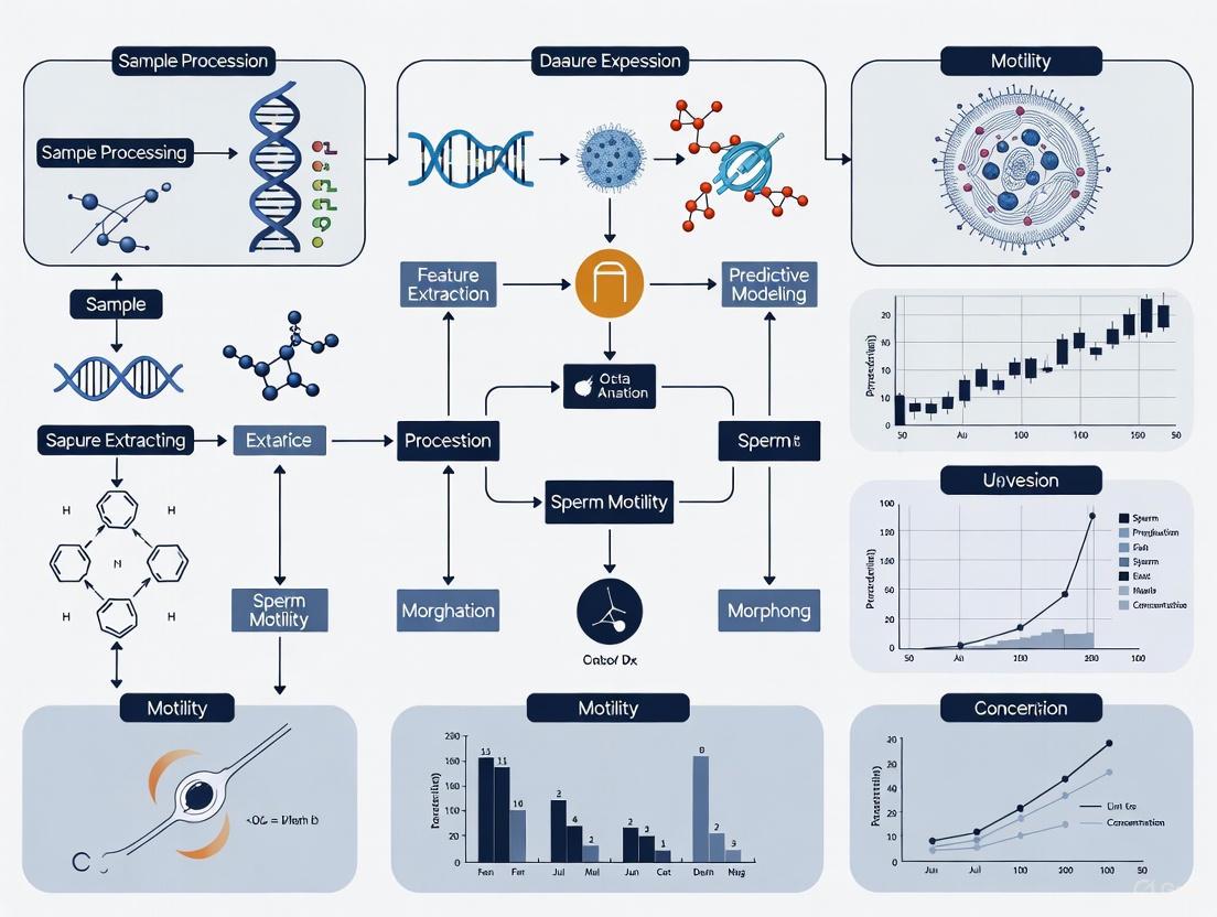
Figure 2: ML-Driven Diagnostic Workflow for Male Infertility. This diagram outlines the integrated process from multidimensional data collection to clinical decision support, highlighting the role of hybrid ML approaches in modern fertility diagnostics.
Application Notes: Core AI Domains in Male Fertility Diagnostics
The integration of Artificial Intelligence (AI) and Machine Learning (ML) is fundamentally transforming the diagnostic landscape in andrology. These technologies introduce objectivity, enhance precision, and uncover complex, multivariate patterns that elude conventional analysis. The table below summarizes the primary applications and documented performance of these data-driven tools.
Table 1: Key Applications and Performance of AI/ML in Male Infertility Diagnostics
| Application Domain | AI/ML Model(s) Used | Reported Performance | Key Advantage |
|---|---|---|---|
| General Fertility Classification | Hybrid MLFFN–ACO (Ant Colony Optimization) [3] | 99% accuracy, 100% sensitivity [3] | Integrates lifestyle/environmental factors; ultra-low computational time (0.00006s) [3]. |
| Sperm Morphology Analysis | Support Vector Machine (SVM), Deep Learning (e.g., TOD-CNN, SHMC-Net) [3] [24] | SVM AUC: 88.59% (1,400 sperm) [18] | Reduces subjectivity; identifies subtle structural variations [3] [25]. |
| Sperm Motility & Kinematics | Computer-Aided Sperm Analysis (CASA) with t-SNE [24] | High predictive accuracy for fertility in models [24] | Provides detailed kinetic variables (velocity, lateral head displacement) [24]. |
| Varicocele Impact Prediction | Deep Neural Network (DNN), Random Forest, XGBoost [26] | DNN Accuracy: 94.1%, Precision: 96.7% [26] | Predicts post-surgical improvement in semen parameters; identifies key cytokines [26]. |
| Sperm Retrieval Prediction (Non-Obstructive Azoospermia) | Gradient Boosted Trees (GBT) [24] [18] | GBT AUC: 0.807, 91% sensitivity [18] | Superior to logistic regression in predicting successful sperm retrieval [24]. |
| IVF Success Prediction | Random Forest, AI-driven platforms [27] [18] | Random Forest AUC: 84.23% [18]; Platform Accuracy: 90% [27] | Integrates clinical, lifestyle, and embryonic data for personalized outcome forecasting [27] [18]. |
Experimental Protocols
Protocol 1: Developing a Hybrid ML Model for Male Fertility Classification
This protocol outlines the methodology for creating a diagnostic framework that combines a Multilayer Feedforward Neural Network (MLFFN) with a nature-inspired Ant Colony Optimization (ACO) algorithm, as demonstrated in recent research [3].
1. Data Acquisition and Preprocessing
- Data Source: Utilize a clinically profiled dataset, such as the publicly available Fertility Dataset from the UCI Machine Learning Repository [3].
- Variables: Ensure the dataset includes a comprehensive set of features: seminal quality (binary outcome: Normal/Altered), socio-demographic data, lifestyle habits (e.g., sedentary behavior, alcohol use), medical history, and environmental exposures [3].
- Data Cleaning: Remove incomplete records. Address class imbalance (e.g., 88 Normal vs. 12 Altered cases) using techniques like oversampling or SMOTE to prevent model bias [3].
- Data Normalization: Apply Min-Max normalization to rescale all features to a [0, 1] range. This ensures consistent contribution from variables originally on different scales (e.g., binary and discrete attributes) and enhances numerical stability during training [3].
2. Model Architecture and Training with ACO
- Base Model: Construct a Multilayer Feedforward Neural Network (MLFFN). The number of layers and neurons should be determined based on the dataset's dimensionality and complexity.
- Integration of ACO: Implement the Ant Colony Optimization algorithm to optimize the MLFFN's learning process. The ACO mimics ant foraging behavior to perform adaptive parameter tuning, enhancing predictive accuracy and overcoming limitations of conventional gradient-based methods. This hybrid strategy (MLFFN–ACO) improves reliability and generalizability [3].
- Proximity Search Mechanism (PSM): Integrate the PSM to provide feature-level interpretability. This mechanism allows the model to highlight the key contributory factors (e.g., sedentary habits, environmental exposures) for each prediction, making the model's decisions clinically interpretable [3].
3. Model Evaluation and Clinical Validation
- Performance Metrics: Evaluate the model on unseen samples using standard metrics: classification accuracy, sensitivity (recall), specificity, and computational time [3].
- Validation: Employ a robust validation method such as k-fold cross-validation. The expected performance for a well-tuned model can be as high as 99% accuracy and 100% sensitivity [3].
- Feature Importance Analysis: Use the integrated PSM or other explainable AI (XAI) techniques like LIME (Local Interpretable Model-agnostic Explanations) to generate clinical interpretability. This analysis emphasizes the weight of each input feature (e.g., lifestyle factors) in the final decision, enabling healthcare professionals to understand and act upon the predictions [3] [26].
Protocol 2: An AI-Driven Workflow for Varicocele Diagnosis and Prognosis
This protocol details the use of ML models to diagnose varicocele and predict its impact on semen quality, incorporating explainable AI for clinical insight [26].
1. Patient Recruitment and Multimodal Data Collection
- Cohort: Recruit patients attending an infertility center for andrological work-up.
- Data Collection: Systematically collect the following data points for each subject:
- Clinical Examination: Findings from a physical examination and testicular ultrasound to confirm the presence and grade of varicocele.
- Semen Analysis: Standard semen parameters (volume, concentration, motility, morphology) following WHO guidelines.
- Advanced Semen Biomarkers: Analyze markers of oxidative stress and inflammation, such as cytokine levels (e.g., IL-17, IL-10, IL-6) in seminal plasma [26].
2. Model Selection and Training for Dual Prediction Tasks
- Objective: Develop models for two distinct supervised prediction tasks:
- Experiment 1 (Predict OAT): Classify the presence of oligoasthenoteratozoospermia (OAT).
- Experiment 2 (Predict VARIX): Diagnose the presence of varicocele.
- Algorithms: Train and compare multiple ML models, including:
- Deep Neural Network (DNN)
- Support Vector Machine (SVM)
- Random Forest (RF)
- XGBoost [26]
- Training: Use a labeled dataset where the targets are the confirmed OAT status and varicocele presence. Employ a train-test split or cross-validation to ensure model generalizability.
3. Model Interpretation using Explainable AI (XAI)
- Integration of LIME: Apply the LIME framework to each trained model. LIME creates local, interpretable approximations of the complex model's behavior for individual predictions [26].
- Feature Importance Extraction: Use LIME to identify which input features (e.g., specific cytokine levels, sperm concentration) had the greatest impact on the model's diagnosis or prognosis for a given patient. This step is crucial for validating the model against clinical knowledge and uncovering potential new biomarkers [26].
The Scientist's Toolkit: Research Reagent Solutions
The following table lists essential materials and computational tools required for implementing AI-driven diagnostics in andrology research.
Table 2: Essential Research Reagents and Tools for AI-Based Andrology Studies
| Item/Tool Name | Type | Primary Function in Research |
|---|---|---|
| Computer-Aided Sperm Analyzer (CASA) | Instrument | Provides automated, high-throughput analysis of sperm concentration, motility, and detailed kinematics; reduces inter-operator variability [24]. |
| Cytokine Profiling Kits (e.g., for IL-17, IL-6, IL-10) | Biochemical Reagent | Quantifies levels of inflammatory cytokines in seminal plasma; used as input features for ML models to diagnose conditions like varicocele and predict semen quality impairment [26]. |
| Sperm DNA Fragmentation (SDF) Assay | Diagnostic Assay | Measures the percentage of sperm with damaged DNA, a known cause of infertility and ART failure. AI models use this data for enhanced diagnostic precision [24] [25]. |
| Ant Colony Optimization (ACO) Library | Computational Tool | A nature-inspired optimization algorithm used to tune hyperparameters of neural networks, enhancing learning efficiency, convergence, and predictive accuracy in diagnostic frameworks [3]. |
| LIME (Local Interpretable Model-agnostic Explanations) | Software Library | An explainable AI (XAI) framework that helps interpret predictions of any complex ML model, building trust and providing clinical insights by highlighting influential input features [26]. |
| FlowJo / Cytobank with ML plugins | Software with AI | Analyzes flow cytometry data at a single-cell level for biofunctional sperm parameters (e.g., mitochondrial membrane potential, oxidative stress) using ML tools like t-SNE and clustering [24]. |
Architecting Intelligence: Core Machine Learning Methodologies for Real-Time Fertility Assessment
The integration of Neural Networks (NN) with bio-inspired optimization algorithms, such as Ant Colony Optimization (ACO), represents a paradigm shift in developing real-time diagnostic systems for male infertility. These hybrid frameworks leverage the powerful pattern recognition capabilities of NNs and the efficient, adaptive search mechanisms of ACO to overcome the limitations of traditional diagnostic methods, which are often prone to subjectivity, low throughput, and an inability to capture complex, non-linear relationships in multifactorial conditions like infertility [12] [14]. The core strength of this synergy lies in using ACO to optimize critical aspects of the neural network, such as feature selection, architecture design, and hyperparameter tuning, thereby enhancing the model's predictive accuracy, convergence speed, and generalizability for clinical use [3] [4].
In the context of male fertility, where etiology encompasses genetic, hormonal, lifestyle, and environmental factors, this integration is particularly valuable. A study demonstrated this by combining a Multilayer Feedforward Neural Network (MLFFN) with ACO to create a hybrid diagnostic model. The ACO algorithm was employed to adaptively tune the parameters of the neural network, mimicking ant foraging behavior to navigate the complex solution space of parameter optimization more effectively than conventional gradient-based methods [4]. This approach resulted in a model that not only achieved high accuracy but also delivered predictions with ultra-low computational time, making it suitable for real-time clinical application [3] [4].
Quantitative Performance of Hybrid Frameworks
The application of hybrid NN-ACO frameworks in male fertility diagnostics has yielded quantitatively superior results compared to standalone machine learning models or traditional statistical approaches. The following table summarizes key performance metrics reported in recent studies.
Table 1: Performance Metrics of AI and Hybrid Models in Male Fertility Diagnostics
| Application Focus | AI/Optimization Technique | Reported Performance Metrics | Dataset/Sample Size |
|---|---|---|---|
| General Fertility Diagnosis | Hybrid MLFFN–ACO Framework [3] [4] | 99% classification accuracy, 100% sensitivity, 0.00006 seconds computational time | 100 clinical male fertility cases [3] [4] |
| Sperm Morphology Analysis | Support Vector Machine (SVM) [12] | AUC of 88.59% | 1,400 sperm images [12] |
| Sperm Motility Analysis | Support Vector Machine (SVM) [12] | 89.9% accuracy | 2,817 sperm analyses [12] |
| Non-Obstructive Azoospermia (NOA) Sperm Retrieval Prediction | Gradient Boosting Trees (GBT) [12] | AUC 0.807, 91% sensitivity | 119 patients [12] |
| IVF Success Prediction | Random Forests [12] | AUC 84.23% | 486 patients [12] |
| Infertility Risk Prediction | Support Vector Machine (SVM) [28] | AUC 96% | 385 patients (329 infertile, 56 fertile) [28] |
| Infertility Risk Prediction | SuperLearner Algorithm [28] | AUC 97% | 385 patients (329 infertile, 56 fertile) [28] |
The data demonstrates that the hybrid MLFFN-ACO framework achieves top-tier performance, particularly in terms of classification accuracy and operational speed, which is a critical requirement for real-time diagnostic systems [3] [4]. Furthermore, the high sensitivity ensures that the model is effective at identifying true positive cases of altered seminal quality, a crucial feature for a diagnostic tool.
Experimental Protocols for a Hybrid NN-ACO Diagnostic System
This section provides a detailed, step-by-step protocol for developing and validating a hybrid NN-ACO framework for male fertility diagnosis, based on established methodologies [3] [4].
Protocol 1: Data Preprocessing and Feature Scaling
Objective: To prepare a clinical fertility dataset for effective model training by handling missing values, encoding categorical variables, and normalizing features. Materials: Raw clinical dataset (e.g., from UCI Machine Learning Repository), Python/R programming environment, libraries (e.g., Pandas, Scikit-learn). Steps:
- Data Loading and Cleaning: Import the dataset. Remove records with incomplete information. The final dataset from a typical study may comprise 100 samples with 10 attributes after cleaning [4].
- Categorical Variable Encoding: Convert categorical variables (e.g., Season, Smoking Habit) into numerical format using one-hot encoding or label encoding.
- Feature Normalization: Apply Min-Max normalization to rescale all numerical features to a [0, 1] range. This is crucial for preventing feature dominance and ensuring numerical stability during NN training. The formula is: ( X_{norm} = \frac{X - X_{min}}{X_{max} - X_{min}} ) where ( X ) is the original value, and ( X_{min} ) and ( X_{max} ) are the feature's minimum and maximum values [4].
- Data Splitting: Split the preprocessed dataset into training (e.g., 70-80%) and testing (e.g., 20-30%) sets, ensuring stratification to maintain the original class distribution (e.g., 88% Normal vs. 12% Altered) in both sets [4] [28].
Protocol 2: Implementing the ACO-based Optimizer
Objective: To implement the ACO algorithm for optimizing the weights and architecture of the neural network. Materials: Normalized training dataset, Python programming environment with NumPy. Steps:
- Parameter Initialization: Define the ACO parameters, including the number of ants in the colony, the maximum number of iterations, pheromone evaporation rate, and the influence of heuristic information.
- Solution Representation: Represent the NN's weights and architectural parameters (e.g., number of hidden neurons) as a path for an ant to traverse. Each node in the graph corresponds to a potential parameter value.
- Pheromone Initialization: Initialize the pheromone trails on all paths to a small constant value.
- Solution Construction: For each ant in the colony, construct a solution (a set of NN parameters) by probabilistically selecting paths based on the pheromone intensity and a heuristic value, which could be inversely related to the anticipated training error.
- Fitness Evaluation: For each ant's solution (parameter set), build and train the NN. Use the classification accuracy on a validation set as the fitness value.
- Pheromone Update:
- Evaporation: Reduce all pheromone values by a fixed evaporation rate.
- Reinforcement: Allow the ants that found the best solutions to deposit pheromone on their paths. The amount of pheromone deposited is proportional to the quality (fitness) of their solution.
- Termination Check: Repeat steps 4-6 until a stopping criterion is met (e.g., a maximum number of iterations or convergence of the solution). The best solution found is the optimized NN parameter set [3] [4].
Protocol 3: Model Training and Validation with Proximity Search
Objective: To train the final neural network with ACO-optimized parameters and validate its performance using robust techniques, incorporating interpretability analysis. Materials: ACO-optimized parameters, preprocessed training and test sets. Steps:
- Network Instantiation: Construct the final MLFFN using the optimized architecture and weight initialization found by the ACO.
- Model Training: Train the network on the full training set. The use of ACO-tuned parameters often leads to faster convergence and avoids the local minima pitfalls of standard backpropagation [4].
- Performance Testing: Evaluate the final model on the held-out test set. Report standard metrics: accuracy, sensitivity (recall), specificity, and precision [3] [4] [28].
- Interpretability Analysis (Proximity Search Mechanism): Implement a Proximity Search Mechanism (PSM) to determine feature importance. This involves systematically perturbing input features and observing the change in the model's output. Features causing significant output deviation when altered are deemed more important for the prediction, thereby providing clinicians with interpretable, feature-level insights [3] [4].
- Cross-Validation: Perform k-fold cross-validation (e.g., 10-fold) to obtain a more reliable estimate of the model's generalization performance and mitigate overfitting [28].
Workflow Visualization
The following diagram illustrates the integrated workflow of the hybrid NN-ACO framework for male fertility diagnostics, from data preparation to clinical interpretation.
The Scientist's Toolkit: Research Reagents & Computational Solutions
The development and validation of hybrid NN-ACO frameworks for male fertility diagnostics rely on a combination of clinical data, specific algorithms, and software tools. The table below details these essential components.
Table 2: Essential Resources for Developing Hybrid NN-ACO Diagnostic Models
| Category | Item/Algorithm | Specification/Function | Reference/Source |
|---|---|---|---|
| Clinical Data | Fertility Dataset | Publicly available dataset from UCI Repository; contains 100 samples with 10 attributes (age, lifestyle, clinical history) for binary classification (Normal/Altered) [4]. | UCI Machine Learning Repository |
| Computational Algorithms | Multilayer Feedforward Neural Network (MLFFN) | Base classifier for pattern recognition; learns non-linear relationships between patient features and fertility status. | [3] [4] |
| Ant Colony Optimization (ACO) | Bio-inspired metaheuristic that optimizes NN parameters (weights, architecture) and performs feature selection. | [3] [4] | |
| Proximity Search Mechanism (PSM) | Explainable AI (XAI) technique for determining feature importance, providing clinical interpretability. | [3] [4] | |
| Support Vector Machine (SVM) | Robust classifier used as a benchmark; effective for high-dimensional spaces and non-linear data. | [12] [28] | |
| SuperLearner Algorithm | Ensemble method that combines multiple algorithms to achieve superior predictive performance. | [28] | |
| Software & Libraries | Python/R | Primary programming environments for implementing machine learning and optimization algorithms. | [28] |
| Scikit-learn, TensorFlow/PyTorch | ML libraries for model building, data preprocessing, and evaluation. | (Implied by standard practice) | |
| Custom ACO/PSM Scripts | Implementation of the specific ACO optimization and interpretability mechanisms. | [3] [4] |
Smartphone-Based Platforms and Portable Devices for Point-of-Care Testing
The integration of smartphone-based platforms and portable devices is revolutionizing point-of-care (POC) testing for male fertility diagnostics. These systems leverage the computational power, connectivity, and imaging capabilities of consumer smartphones to provide clinical-grade semen analysis outside traditional laboratory settings. By incorporating machine learning (ML) algorithms and computer vision techniques, these platforms automate the assessment of key sperm parameters such as concentration and motility with accuracy comparable to computer-assisted semen analysis (CASA) systems [29]. This technological approach addresses significant barriers in male fertility evaluation, including psychological discomfort associated with clinical visits and the limited availability of specialized andrology laboratories [29] [30]. Recent advancements have demonstrated strong correlation with laboratory standards, with one smartphone method achieving Spearman rank correlation coefficients of 0.94 for concentration and 0.89 for motility in clinical tests involving 50 participants [29].
Performance Comparison of Testing Modalities
Table 1: Analytical Performance of Smartphone-Based Semen Analysis Platforms
| Platform/Study | Key Technology | Sperm Parameters Measured | Accuracy/Correlation | Clinical Validation |
|---|---|---|---|---|
| Automated POC Semen Analysis [29] | Smartphone imaging, Occlusion-aware Multi-Object Tracking | Concentration, Motility | Mean error: 2.03 million/mL (concentration), 1.58% (motility); 95.14% success tracking occluded sperm | 50 participants; Spearman correlation: 0.94 (conc.), 0.89 (motility) |
| Remote Smartphone-Based Assessment [31] | Smartphone-based analyzer, delayed CASA | Concentration, Total Motility | High specificity (86.2%), NPV (93.8%) for low concentration; Highly reproducible (ICC: 0.98 conc., 0.90 motility) | 92 men; Prospective study; Comparison to lab CASA |
| YO Home Sperm Test [32] | Smartphone-based video analysis, disposable test device | Concentration, Motility, Progressive Motility, Motile Sperm Concentration, Progressive Motile Sperm Concentration | >97% accuracy; FDA-cleared; WHO 6th Edition compliant | Doctor-recommended; Clinical-grade results |
Table 2: Operational Characteristics of Point-of-Care Male Fertility Tests
| Characteristic | Smartphone Microscopic Imaging [29] | Remote Smartphone Analyzer [31] | YO Home Sperm Test [32] |
|---|---|---|---|
| Testing Environment | Point-of-Care | Home | Home |
| Sample Processing | Undiluted raw semen | Remote collection | At-home collection, no mail-in |
| Analysis Time | Real-time tracking | N/A (requires sample shipping) | < 20 minutes |
| Key ML/Software Features | Occlusion-aware multi-sperm tracking, boundary-sensitive segmentation | Not specified | Live video recording, automated analysis |
| Result Delivery | Smartphone display | Not specified | Smartphone app, PDF report |
| Regulatory Status | Research phase | Research phase | FDA-cleared |
Experimental Protocols
Protocol: Smartphone-Based Semen Analysis with Occlusion-Aware Tracking
This protocol outlines the procedure for using a smartphone-based imaging system to assess sperm concentration and motility, incorporating ML algorithms for robust tracking [29].
Materials and Equipment
- Smartphone with high-resolution camera and dedicated application software
- Custom optical attachment for microscopic imaging
- Disposable sample chamber (e.g., counting chamber slide)
- Fresh, undiluted semen sample (collected per standard clinical guidelines)
- Data processing unit (smartphone or connected computer) with ML tracking algorithm
Procedure
- Sample Preparation: Collect semen sample via masturbation after a recommended 2-5 days of sexual abstinence. Allow the sample to liquefy completely at room temperature for 20-30 minutes. Do not dilute the sample.
- Device Setup: Attach the custom optical lens to the smartphone camera, ensuring a secure fit. Launch the semen analysis application on the smartphone.
- Loading: Pipette a small volume (approximately 5-10 µL) of the liquefied semen sample into the disposable counting chamber. Carefully place the chamber under the smartphone-based imaging module, ensuring proper contact and alignment.
- Image Acquisition: Initiate video recording through the application. Capture multiple video sequences from different fields of view within the chamber. Ensure stable positioning to minimize motion artifacts. The recommended video duration is 30-60 seconds per field to adequately assess motility.
- ML-Based Analysis: The application automatically processes the video using the following computational workflow:
- Segmentation: A boundary-sensitive segmentation network identifies and distinguishes sperm cells from impurities and background debris in the raw semen.
- Occlusion Handling: An occlusion-awareness module combines contour information and kinematic-based probabilistic modeling to detect and manage sperm crossover and occlusion events.
- Multi-Object Tracking: A multi-sperm tracking algorithm follows individual sperm trajectories across frames, even during frequent occlusion events.
- Parameter Calculation: The algorithm calculates sperm concentration (million/mL), total motility (%), and progressive motility (%) based on the segmented and tracked cells.
- Result Interpretation: Review the generated report on the smartphone screen. The report includes quantitative values for key parameters and may flag samples below WHO reference limits for clinical review.
Protocol: Validation Against Laboratory CASA Systems
This protocol describes the method for validating the performance of a smartphone-based semen analyzer against a laboratory-grade CASA system as a reference standard [31].
Materials and Equipment
- Smartphone-based semen analyzer (commercial or research prototype)
- Standard laboratory CASA system
- Semen samples from recruited participants (e.g., men unselected for fertility status)
- Sample collection kits including sterile containers
- Data management system for result comparison
Procedure
- Participant Recruitment and Sample Collection: Recruit a cohort of participants (e.g., n=150) representing the general population, not selected based on fertility concerns. Provide standardized instructions for semen collection.
- Split-Sample Analysis: For each participant:
- Arm A (Smartphone Analysis): Immediately after liquefaction, analyze a portion of the sample using the smartphone-based platform according to the manufacturer's instructions.
- Arm B (Laboratory Analysis): Preserve the remaining portion of the sample in appropriate conditions and transport it to the andrology laboratory for analysis. Record the time elapsed between collection and laboratory analysis (e.g., target <30 hours).
- Laboratory Assessment: Analyze the sample using the laboratory CASA system following standardized operational protocols. Mask the laboratory technicians to the results of the smartphone analysis.
- Data Comparison: Statistically compare the key parameters (sperm concentration and total motility) obtained from both methods.
- Agreement Analysis: Use Bland-Altman plots to visualize the agreement and identify any bias between the two methods.
- Reproducibility: Calculate intraclass correlation coefficients (ICC) to assess the reproducibility of the smartphone-based measures.
- Diagnostic Performance: Calculate specificity and negative predictive value (NPV) of the smartphone system for identifying samples with low sperm concentration (e.g., <16 million/mL) as defined by the laboratory standard.
Visualization of Workflows
Smartphone-Based Semen Analysis Workflow
ML Algorithm Processing Pipeline
The Scientist's Toolkit: Research Reagent Solutions
Table 3: Essential Materials for Smartphone-Based Male Fertility Research
| Item | Function/Application | Specification Notes |
|---|---|---|
| Smartphone with Camera | Core imaging device for video capture | High-resolution camera (e.g., ≥12 MP); Capable of continuous video recording |
| Custom Optical Attachment | Microscopic magnification for sperm visualization | Provides sufficient magnification to resolve individual sperm cells (e.g., ~10-20x) |
| Disposable Sample Chambers | Hold semen sample for analysis | Standardized depth (e.g., 10-20 µm); Low adhesion surface to minimize trapping |
| ML-Enabled Software | Automated sperm identification and tracking | Implements segmentation and occlusion-aware algorithms; Provides quantitative output |
| Reference CASA System | Gold-standard validation of new methods | Laboratory-grade computer-assisted semen analyzer for performance comparison |
| Data Processing Unit | Runs computational analysis | Smartphone itself or connected external computer/cloud service |
Male infertility, a contributing factor in nearly half of all infertility cases, is a complex condition influenced by a multifaceted interplay of clinical, lifestyle, and environmental parameters [33]. Traditional diagnostic methods, primarily based on standard semen analysis, often fail to capture this complexity, leading to a high prevalence of idiopathic diagnoses [34] [35]. The integration of machine learning (ML) into male fertility diagnostics offers a paradigm shift, enabling the development of predictive, real-time diagnostic systems. The efficacy of these ML models is fundamentally dependent on robust feature engineering—the process of selecting, constructing, and transforming raw input variables to enhance model performance. This protocol details the methodology for engineering a comprehensive feature set that accurately reflects the multifactorial nature of male infertility, tailored for high-precision, real-time diagnostic systems.
Parameter Categorization and Quantitative Data Synthesis
A critical first step in feature engineering is the systematic identification and categorization of relevant parameters from heterogeneous data sources. The table below synthesizes key parameter types, their specific features, and their documented impact on semen quality, providing a structured framework for data collection.
Table 1: Categorization and Impact of Male Fertility Parameters
| Parameter Category | Specific Features | Impact on Semen Quality & Key Findings |
|---|---|---|
| Clinical & Semen Parameters | Volume, Concentration, Motility, Morphology, Sperm Mitochondrial DNA Copy Number (mtDNAcn), DNA Fragmentation Index (DFI) | mtDNAcn is a top predictive biomarker for pregnancy at 12 cycles (AUC: 0.68). A composite ML index including mtDNAcn achieved an AUC of 0.73 [36]. High DFI impairs sperm function [33]. |
| Lifestyle Factors | Smoking Habit, Alcohol Consumption, Sitting Hours Per Day, Obesity, Physical Activity Level | Smoking reduces sperm concentration, motility, and morphology, and increases DNA fragmentation [35]. Prolonged sitting is a key contributory factor identified by feature-importance analysis [3] [4]. Moderate exercise improves sperm concentration and motility, while excessive exercise can be detrimental [35]. |
| Environmental Exposures | Air Pollution (PM2.5, PM10), Endocrine Disruptors (Bisphenols, Phthalates), Heavy Metals, Pesticides | Exposure to PM2.5 and SO2 is negatively correlated with semen quality. Improvement in air quality in Wenzhou, China, was associated with increased progressive motility, total motility, and semen volume [37]. Environmental factors are main hormonal disruptors, primarily acting via oxidative stress [34]. |
| Psychological & Sociodemographic | Psychosocial Stress, Age, Occupation, Education Level | Heightened stress, anxiety, and depression are linked to infertility. Older age and certain occupations (e.g., workers) are associated with significantly worse semen quality [3] [37]. |
Experimental Protocols for Integrated Feature Engineering
Protocol: Data Preprocessing and Normalization
Objective: To transform raw, heterogeneous data into a clean, normalized dataset suitable for machine learning models.
Materials:
- Raw clinical, lifestyle, and environmental dataset (e.g., from UCI Fertility Dataset) [3] [4].
- Computational environment (e.g., Python with Scikit-learn library).
Methodology:
- Data Cleaning: Handle missing values using imputation strategies (e.g., mean/median for continuous, mode for categorical) or removal of incomplete records.
- Range Scaling (Normalization): Apply Min-Max normalization to rescale all features to a [0, 1] range. This is crucial when parameters have heterogeneous scales (e.g., age in years, sitting hours per day, and binary features like smoking habit).
- Handling Class Imbalance: For datasets with a skewed class distribution (e.g., 88 "Normal" vs. 12 "Altered" semen quality cases), employ techniques such as Synthetic Minority Over-sampling Technique (SMOTE) to prevent model bias toward the majority class [3] [4].
Protocol: Hybrid Feature Selection using Bio-Inspired Optimization
Objective: To identify the most discriminative subset of features to enhance model accuracy and generalizability while reducing computational overhead for real-time application.
Materials:
- Preprocessed and normalized fertility dataset.
- Machine Learning framework (e.g., Python) with Ant Colony Optimization (ACO) library.
Methodology:
- Algorithm Selection: Implement a hybrid framework combining a Multilayer Feedforward Neural Network (MLFFN) with an Ant Colony Optimization (ACO) algorithm. ACO is a nature-inspired metaheuristic that mimics ant foraging behavior for efficient pathfinding, which is analogous to optimal feature subset selection [3] [4].
- Proximity Search Mechanism (PSM): Integrate PSM to provide feature-level interpretability. This mechanism evaluates the contribution of each feature to the final classification, allowing clinicians to understand which factors (e.g., sedentary hours, environmental exposures) are most influential in the diagnosis [3] [4].
- Model Training & Evaluation:
- The ACO algorithm is used for adaptive parameter tuning and feature selection within the MLFFN.
- The model is trained and evaluated using k-fold cross-validation.
- Performance Metrics: Assess classification accuracy, sensitivity (recall), specificity, and computational time on unseen samples. The cited study achieved 99% accuracy, 100% sensitivity, and an ultra-low computational time of 0.00006 seconds, demonstrating real-time feasibility [3] [4].
Protocol: Deep Feature Engineering for Sperm Image Analysis
Objective: To extract high-dimensional, discriminative features from sperm microscopy images for automated morphology classification.
Materials:
- Sperm image datasets (e.g., SMIDS, HuSHeM).
- Pre-trained Convolutional Neural Network (CNN) models (e.g., ResNet50) enhanced with a Convolutional Block Attention Module (CBAM).
- Feature selection methods (e.g., PCA, Chi-square test, Random Forest importance).
Methodology:
- Backbone Feature Extraction: Use a CBAM-enhanced ResNet50 architecture to process sperm images. The CBAM module allows the network to focus on morphologically relevant regions (e.g., head shape, acrosome, tail) while suppressing background noise [38].
- Deep Feature Pooling: Extract deep feature embeddings from multiple layers of the network, including Global Average Pooling (GAP) and Global Max Pooling (GMP) layers [38].
- Dimensionality Reduction & Classification: Apply Principal Component Analysis (PCA) to the high-dimensional deep features to reduce noise and redundancy. Subsequently, train a shallow classifier (e.g., Support Vector Machine with RBF kernel) on the reduced feature set. This hybrid CNN+DFE approach has been shown to achieve state-of-the-art accuracy of 96.08% on benchmark datasets [38].
Visualization of Workflows and Signaling Pathways
Integrated Feature Engineering and Model Training Workflow
Signaling Pathway of Environmental Stressors on Sperm Quality
The Scientist's Toolkit: Research Reagent Solutions
Table 2: Essential Research Reagents and Materials for Male Fertility ML Research
| Item Name | Function/Application |
|---|---|
| LensHooke X1 PRO | An AI-powered optical microscopic system for automated semen analysis, providing high correlation with manual methods for concentration and progressive motility [33]. |
| Sperm DNA Fragmentation Assay Kits | Used to measure DNA Fragmentation Index (DFI), a key biomarker of sperm genetic integrity that is predictive of fertilization success and embryo health [33]. |
| Antioxidant Supplements (e.g., CoQ10, Vitamins C & E, Zinc, Selenium) | Used in clinical trials to investigate the reduction of oxidative stress and its subsequent improvement on sperm concentration, motility, and morphology [39] [35]. |
| Publicly Available Fertility Datasets (e.g., UCI Fertility Dataset) | Provide structured, real-world data encompassing clinical, lifestyle, and environmental parameters for training and validating machine learning models [3] [4]. |
| Pre-trained CNN Models (e.g., ResNet50, Xception) | Serve as backbone architectures for transfer learning and deep feature extraction from sperm images, significantly reducing the need for large, labeled datasets and computational resources [38]. |
| Ant Colony Optimization (ACO) Library | Computational tool for implementing nature-inspired optimization algorithms for feature selection and hyperparameter tuning in machine learning pipelines [3] [4]. |
Explainable AI (XAI) and Feature-Importance Analysis for Clinical Interpretability
The integration of Artificial Intelligence (AI) into male fertility diagnostics promises enhanced precision but also introduces the challenge of the "black box" phenomenon, where model decisions are opaque. Explainable AI (XAI) addresses this by making AI decisions transparent, interpretable, and trustworthy for clinicians. Within real-time male fertility diagnostic systems, XAI transforms complex model outputs into clinically actionable insights, enabling healthcare professionals to understand the why behind a prediction. This is critical for moving from a paradigm of automated decision-making to one of AI-assisted clinical reasoning, where models not only predict but also elucidate the contributing factors—such as lifestyle, environmental, and clinical parameters—to male infertility. This document provides a detailed overview of prominent XAI techniques, their performance in male fertility applications, and standardized protocols for their implementation, specifically tailored for researchers and scientists developing diagnostic systems.
Key XAI Techniques and Their Clinical Application in Male Fertility
In male fertility diagnostics, several XAI techniques have been successfully applied to interpret complex machine learning models. The table below summarizes the core techniques, their methodological approach, and clinical application.
Table 1: Key Explainable AI (XAI) Techniques in Male Fertility Diagnostics
| XAI Technique | Methodological Approach | Clinical Application & Interpretation |
|---|---|---|
| SHapley Additive exPlanations (SHAP) [40] [41] | A game-theory based approach that assigns each feature an importance value for a particular prediction. It computes the marginal contribution of a feature across all possible combinations of features. | Global Interpretability: Ranks features (e.g., female age, testicular volume, FSH levels) by their overall impact on model output [41]. Local Interpretability: Explains individual predictions, showing how each factor pushed the model's output towards "Altered" or "Normal" fertility [40]. |
| Local Interpretable Model-agnostic Explanations (LIME) [40] [26] | Approximates a complex model locally around a specific prediction by creating a simpler, interpretable model (e.g., linear model) on a perturbed sample of the instance. | Provides "case-by-case" explanations that are easily understandable to clinicians. For example, it can highlight that a specific patient's prediction of oligoasthenoteratozoospermia (OAT) was primarily driven by elevated levels of a specific cytokine [26]. |
| Feature Importance (e.g., ELI5, XGBoost Built-in) [40] [11] | Ranks features based on a metric quantifying their usefulness in making accurate predictions (e.g., how often a feature is used to split data in tree-based models). | Offers a macro-level view of predictive factors. Studies have used this to identify that follicle-stimulating hormone (FSH), inhibin B, and testicular volume are top predictors for azoospermia, while environmental factors like PM10 and NO2 are crucial for semen quality alterations [11]. |
| Proximity Search Mechanism (PSM) [3] | A bio-inspired optimization technique that provides feature-level insights by adapting parameters based on problem structure, akin to ant foraging behavior. | Integrated with neural networks, it enhances model interpretability by identifying and ranking key contributory lifestyle and environmental risk factors, such as sedentary habits, for a specific diagnosis [3]. |
Quantitative Performance of XAI-Empowered Models
The application of XAI is often coupled with high-performing predictive models. The following table summarizes the demonstrated efficacy of various AI/XAI frameworks in male fertility research, providing a benchmark for expected performance.
Table 2: Performance Metrics of AI/XAI Models in Male Fertility Studies
| Study & Model | Key Features / XAI Technique | Dataset | Performance Metrics |
|---|---|---|---|
| Hybrid MLFFN–ACO Framework [3] | Ant Colony Optimization (ACO) for adaptive parameter tuning; Proximity Search Mechanism (PSM) for interpretability. | 100 male fertility cases from UCI Repository [3] | Accuracy: 99% Sensitivity: 100% Computational Time: 0.00006 seconds [3] |
| XGBoost with SHAP/LIME [40] | Extreme Gradient Boosting; explained with SHAP and LIME for local and global interpretability. | Lifestyle and environmental factors dataset [40] | AUC: 0.98 [40] |
| XGBoost with SHAP [41] | XGBoost for prediction; SHAP for global and local interpretation of clinical pregnancy outcomes. | 345 infertile couples undergoing ICSI [41] | AUROC: 0.858 Accuracy: 79.71% [41] |
| XGBoost for Azoospermia Prediction [11] | XGBoost with built-in feature importance (F-score). | UNIROMA dataset (2,334 men) [11] | AUC: 0.987 Top Features: FSH (F-score=492), Inhibin B (F-score=261), Testicular Volume (F-score=253) [11] |
| Deep Neural Network (DNN) with LIME [26] | DNN for high-accuracy prediction; LIME for explaining predictions of OAT and varicocele. | Clinical and cytokine data from infertility patients [26] | Accuracy (OAT prediction): 0.98 Precision (OAT prediction): 1.0 Recall (OAT prediction): 0.867 [26] |
Experimental Protocol for Implementing XAI in Fertility Diagnostics
This section provides a detailed, step-by-step protocol for developing, validating, and interpreting an XAI-based male fertility diagnostic model, based on methodologies consolidated from the literature [3] [40] [41].
Data Preprocessing and Feature Engineering
Objective: To prepare a clean, normalized, and well-structured dataset for model training.
- Data Sourcing: Utilize a publicly available dataset, such as the UCI Fertility Dataset (100 samples, 10 attributes) [3], or collect retrospective clinical data encompassing semen parameters, hormonal assays (FSH, Testosterone, Inhibin B), lifestyle factors, and environmental exposures [41] [11].
- Handling Missing Values: For features with <10% missing data, use ML-based imputation methods like the missForest algorithm (Random Forest-based) to predict and fill missing values [41].
- Data Normalization: Apply Min-Max Normalization to rescale all continuous features to a [0, 1] range. This ensures features on different scales contribute equally to the model [3] [41].
- Formula: ( X{\text{norm}} = \frac{X - X{\min}}{X{\max} - X{\min}} )
- Addressing Class Imbalance: If the dataset is imbalanced (e.g., more "Normal" than "Altered" cases), apply synthetic oversampling techniques such as the Synthetic Minority Over-sampling Technique (SMOTE) to generate synthetic samples of the minority class [40].
- Feature Selection: Use Recursive Feature Elimination (RFE) or model-specific importance scores to remove redundant features and mitigate multicollinearity, retaining the most predictive feature set [41].
Model Training and Validation
Objective: To build a robust predictive model using state-of-the-art algorithms.
- Algorithm Selection: Choose one or more of the following high-performing algorithms:
- XGBoost (Extreme Gradient Boosting): An ensemble tree-based method known for high accuracy and speed [40] [41] [11].
- Hybrid Neural Network with ACO: A multilayer feedforward neural network integrated with the Ant Colony Optimization algorithm for enhanced learning and convergence [3].
- Deep Neural Network (DNN): For complex, high-dimensional data, a DNN can capture intricate non-linear relationships [26].
- Random Forest (RF): An ensemble method effective for classification and providing inherent feature importance metrics [26].
- Hyperparameter Tuning: Perform a randomized or grid search with 5-fold cross-validation to fine-tune model hyperparameters (e.g., learning rate, tree depth, number of estimators) for optimal performance [40] [11].
- Model Validation: Split the data into training (e.g., 70-80%) and testing (e.g., 20-30%) sets. Use hold-out validation or k-fold cross-validation (k=5 is standard) to assess model generalizability [40]. Report standard metrics including Accuracy, AUC, Precision, Recall, F1-Score, and Brier Score [41].
Model Interpretation via XAI
Objective: To deconstruct the model's predictions and derive clinically meaningful insights.
- Global Interpretability with SHAP:
- Fit a SHAP explainer (e.g.,
shap.TreeExplainerfor XGBoost) to the trained model. - Generate a summary plot (shap.summary_plot) that displays the mean absolute SHAP value for each feature, ranking them by their overall importance in the model's predictions [40] [41].
- This identifies the "big picture" drivers of fertility outcomes across the entire population.
- Fit a SHAP explainer (e.g.,
- Local Interpretability with SHAP/LIME:
- For a specific patient's prediction, use SHAP force plots (
shap.force_plot) or LIME explanations to visualize how each feature contributed to the final output for that individual. - The output shows features that pushed the prediction higher (e.g., towards "Altered") and those that pushed it lower, along with their magnitude [40] [26].
- This is crucial for personalized patient counseling and intervention planning.
- For a specific patient's prediction, use SHAP force plots (
- Feature Importance Analysis:
- For tree-based models like XGBoost and Random Forest, extract and plot the built-in feature importance scores (e.g.,
model.feature_importances_), often based on the "F-score" metric (number of times a feature is used to split the data) [11]. - This provides a complementary view to SHAP for validating the top predictive features.
- For tree-based models like XGBoost and Random Forest, extract and plot the built-in feature importance scores (e.g.,
The following diagram illustrates the end-to-end workflow of this protocol, from data preparation to clinical interpretation.
Signaling Pathways from Model Output to Clinical Decision
The interpretable outputs generated by XAI must be mapped to a logical clinical decision pathway. The diagram below visualizes this flow, demonstrating how a model's prediction and its accompanying explanation guide clinical action.
The Scientist's Toolkit: Research Reagent Solutions
For researchers aiming to replicate or build upon the described methodologies, the following table details essential computational tools and their functions as utilized in the cited studies.
Table 3: Essential Research Tools for XAI Implementation in Male Fertility
| Tool / Reagent | Type | Function in Protocol | Exemplar Use Case |
|---|---|---|---|
| XGBoost Library [40] [41] [11] | Software Library | Primary model for high-accuracy prediction; provides built-in feature importance. | Predicting clinical pregnancy from surgical sperm retrieval parameters [41]. |
| SHAP Library [40] [41] | Software Library | Post-hoc model interpretation for both global and local explainability. | Identifying female age and testicular volume as top features for pregnancy success [41]. |
| LIME Library [40] [26] | Software Library | Creating local, interpretable surrogate models to explain individual predictions. | Explaining a DNN's prediction of OAT based on a patient's cytokine profile [26]. |
| SMOTE [40] | Data Preprocessing Algorithm | Synthetically generating samples of the minority class to balance dataset. | Handling the imbalance between "Normal" and "Altered" fertility classes [40]. |
| Ant Colony Optimization (ACO) [3] | Optimization Algorithm | Tuning neural network parameters adaptively to enhance learning and convergence. | Powering a hybrid diagnostic framework for ultra-fast and accurate fertility classification [3]. |
Male infertility is a pressing global health issue, contributing to nearly 50% of all infertility cases among couples, yet it often remains underdiagnosed due to limitations in traditional diagnostic methods [3] [18]. Conventional approaches like semen analysis, while foundational, are often subjective, time-consuming, and fail to capture the complex interplay of clinical, lifestyle, and environmental factors influencing reproductive health [42] [11] [18]. This diagnostic gap has created an urgent need for innovative, data-driven solutions.
Artificial intelligence (AI) and machine learning (ML) are now revolutionizing male fertility diagnostics by enabling the analysis of complex, multifactorial data with unprecedented precision [42] [33]. This case study explores a groundbreaking hybrid diagnostic framework that integrates a Multilayer Feedforward Neural Network (MLFFN) with a nature-inspired Ant Colony Optimization (ACO) algorithm. This system was developed to enhance predictive accuracy, overcome the limitations of conventional gradient-based methods, and provide a robust, generalizable, and efficient tool for real-time male fertility assessment [3].
State of the Field: AI in Male Infertility
The application of AI in male infertility is a rapidly advancing field. A recent systematic review of ML models for predicting male infertility reported a median accuracy of 88% across 43 studies, with Artificial Neural Networks (ANNs) specifically achieving a median accuracy of 84% [42]. AI's utility spans several critical areas:
- Sperm Analysis: Deep learning models automate and enhance the evaluation of sperm morphology, motility, and concentration, achieving accuracies exceeding 90% in classifying sperm and reducing inter-observer variability [18] [33].
- Severe Infertility Treatment: For conditions like azoospermia, novel systems like the Sperm Tracking and Recovery (STAR) method use AI to identify and recover viable sperm from samples previously considered devoid of sperm, enabling successful pregnancies in previously untreatable cases [43] [44].
- Fertilisation Potential Prediction: AI models can now evaluate sperm morphology based on its ability to bind to the zona pellucida (the egg's outer layer), predicting fertilisation competence with over 96% accuracy [45].
These advancements highlight a paradigm shift towards more objective, efficient, and accurate diagnostic tools. However, challenges remain in handling class imbalance in medical datasets and improving model generalizability, which the MLFFN-ACO framework directly addresses [3].
Methodology and Experimental Protocols
Dataset Description and Preprocessing
The framework was developed and evaluated using a publicly available Fertility Dataset from the UCI Machine Learning Repository, comprising 100 clinically profiled male fertility cases from volunteers aged 18-36 [3].
Key Dataset Characteristics:
- Attributes: 10 features encompassing socio-demographic, lifestyle, medical history, and environmental exposure factors.
- Output: Binary classification of seminal quality as "Normal" or "Altered."
- Class Distribution: 88 "Normal" and 12 "Altered" cases, presenting a moderate class imbalance that the model was designed to handle.
Preprocessing Protocol:
- Data Cleaning: Removal of incomplete records to ensure data integrity.
- Normalization: All features were rescaled to a [0, 1] range using Min-Max normalization to ensure consistent contribution and prevent scale-induced bias, despite some features being initially binary (0, 1) or discrete (-1, 0, 1) [3]. The formula is given by: ( X{\text{norm}} = \frac{X - X{\min}}{X{\max} - X{\min}} )
The Hybrid MLFFN-ACO Framework Architecture
The core innovation lies in synergistically combining a Multilayer Feedforward Neural Network (MLFFN) with the Ant Colony Optimization (ACO) algorithm.
Table: Core Components of the Hybrid MLFFN-ACO Framework
| Component | Description | Primary Function |
|---|---|---|
| Multilayer Feedforward Neural Network (MLFFN) | A standard neural network architecture with an input layer, hidden layers, and an output layer. | To learn complex, non-linear relationships between the input clinical/lifestyle factors and the fertility outcome. |
| Ant Colony Optimization (ACO) | A nature-inspired metaheuristic algorithm that mimics ant foraging behavior for pathfinding. | To perform adaptive parameter tuning and feature selection, optimizing the MLFFN's weights and architecture to enhance learning efficiency and convergence. |
| Proximity Search Mechanism (PSM) | An interpretability component integrated into the framework. | To provide feature-level importance analysis, highlighting key contributory factors (e.g., sedentary habits) for clinical decision-making. |
ACO Optimization Protocol:
- Problem Representation: The search for optimal neural network parameters is modeled as a graph where paths represent potential solutions.
- Solution Construction: "Artificial ants" traverse the graph, building solutions (parameter sets) probabilistically, biased by "pheromone" levels and heuristic information.
- Pheromone Update: Paths corresponding to high-performance solutions (e.g., low classification error) receive stronger pheromone deposits, reinforcing their selection in subsequent iterations.
- Integration with MLFFN: The AO-optimized parameters are used to train the MLFFN, overcoming local minima and accelerating convergence compared to traditional backpropagation [3].
Workflow Visualization
The following diagram illustrates the integrated workflow of the hybrid MLFFN-ACO framework for male fertility diagnosis.
Evaluation Metrics Protocol
Model performance was rigorously assessed on unseen samples using standard classification metrics:
- Accuracy: (True Positives + True Negatives) / Total Predictions
- Sensitivity (Recall): True Positives / (True Positives + False Negatives)
- Computational Time: Measured from prediction initiation to result output.
Results and Performance Analysis
The hybrid MLFFN-ACO framework demonstrated exceptional performance in diagnosing male fertility, achieving benchmarks that underscore its potential for real-world clinical application.
Table: Performance Summary of the Hybrid MLFFN-ACO Framework
| Metric | Result | Significance |
|---|---|---|
| Classification Accuracy | 99% | Surpasses the reported median accuracy (88%) of other ML models in male infertility prediction [42]. |
| Sensitivity | 100% | Excellent at identifying all true "Altered" cases, crucial for a diagnostic test to avoid missing at-risk individuals. |
| Computational Time | 0.00006 seconds | Enables real-time diagnostics, facilitating immediate clinical decision-making. |
The 99% classification accuracy significantly exceeds the performance of many existing models, as identified in a recent literature review [42]. Furthermore, the achievement of 100% sensitivity is particularly critical in a medical context, as it ensures that individuals with altered fertility are not incorrectly classified as normal. The framework's ultra-low computational time highlights its efficiency and suitability for integration into clinical workflows where rapid results are essential [3].
The Scientist's Toolkit: Research Reagent Solutions
The experimental implementation of such a hybrid framework relies on both computational tools and specific datasets.
Table: Essential Research Materials and Resources
| Item | Function / Description | Relevance in the MLFFN-ACO Study |
|---|---|---|
| Fertility Dataset (UCI Repository) | A curated dataset of 100 male fertility cases with 10 clinical, lifestyle, and environmental attributes. | Served as the foundational data for model training, testing, and validation [3]. |
| Ant Colony Optimization (ACO) Library | Software libraries (e.g., in Python, MATLAB) that implement the ACO metaheuristic for optimization tasks. | Crucial for developing the optimization component that tunes the MLFFN parameters [3]. |
| Neural Network Framework | Platforms such as TensorFlow, PyTorch, or scikit-learn for constructing and training MLP/MLFFN models. | Provided the infrastructure for building the core classifier of the hybrid framework [3]. |
| High-Speed Computational Hardware | Computing systems with sufficient CPU/GPU resources to handle iterative training and optimization processes. | Necessary to achieve the reported ultra-low computational time of 0.00006 seconds for real-time analysis [3]. |
Implementation Protocols for Real-Time Diagnostics
Model Training and Validation Protocol
For researchers seeking to replicate or build upon this work, the following detailed protocol is provided:
Data Acquisition and Preparation:
- Source the "Fertility Dataset" from the UCI Machine Learning Repository.
- Execute the preprocessing protocol: remove incomplete entries and apply Min-Max normalization to scale all features to the [0,1] range.
Model Configuration and Training:
- Initialize the MLFFN: Define an architecture with an input layer (nodes = number of features), one or more hidden layers, and an output layer (1 node for binary classification).
- Initialize the ACO: Set ACO parameters (number of ants, evaporation rate, heuristic influence) to govern the search for optimal MLFFN weights.
- Hybrid Training Loop:
- The AO module generates candidate solutions (weight sets).
- Each solution is evaluated by training the MLFFN and measuring performance (e.g., accuracy on a validation set).
- ACO updates pheromone trails based on solution quality.
- Iterate until convergence criteria are met (e.g., max iterations or performance plateau).
Model Validation and Interpretation:
- Evaluate the final model on a held-out test set to obtain unbiased performance metrics (accuracy, sensitivity).
- Run the Proximity Search Mechanism (PSM) on the trained model to compute and output feature importance scores, identifying key predictive factors like sedentary behavior and environmental exposures [3].
System Integration Workflow
The operational workflow for deploying the trained model in a real-time diagnostic setting is visualized below.
This case study demonstrates that the hybrid MLFFN–ACO framework represents a significant leap forward for male fertility diagnostics. By achieving 99% accuracy, 100% sensitivity, and real-time processing speeds, it directly addresses critical limitations of traditional and standalone ML methods. The integration of AO for optimization ensures robust performance, while the Proximity Search Mechanism provides much-needed clinical interpretability.
This framework holds immense promise for reducing diagnostic burden, enabling early detection, and supporting personalized treatment planning. Future work should focus on external validation with larger, multi-center datasets and further exploration of its integration into clinical decision support systems to fully realize its potential in improving male reproductive healthcare.
Navigating Development Hurdles: Data, Generalization, and Clinical Integration Challenges
Addressing Class Imbalance in Medical Datasets for Rare Outcomes
Class imbalance remains a significant challenge in developing machine learning (ML) models for medical diagnostics, particularly for predicting rare outcomes. In male fertility diagnostics, this issue is frequently encountered where datasets often contain a majority of "normal" semen quality cases and a minority of clinically significant "altered" cases [3]. Conventional ML algorithms trained on such imbalanced data tend to be biased toward the majority class, resulting in poor detection of the minority class that often represents the critical medical condition requiring identification [46] [47].
This protocol outlines comprehensive methodologies for addressing class imbalance in medical datasets, with specific application to male fertility diagnostics. We present a systematic framework encompassing data-level, algorithm-level, and hybrid approaches, along with experimental protocols and implementation guidelines tailored for researchers developing real-time male fertility diagnostic systems.
Background and Significance
In medical diagnostics, the minority class (e.g., patients with fertility issues) is typically the class of primary interest, despite being underrepresented in datasets. The imbalance ratio (IR), calculated as IR = Nmaj/Nmin, where Nmaj and Nmin represent the number of instances in the majority and minority classes respectively, quantifies the severity of this disproportion [46]. High IR values present substantial challenges for classification algorithms.
In male fertility studies, datasets often exhibit moderate to severe imbalance. For instance, one fertility dataset contained 88 normal cases versus 12 altered cases (IR ≈ 7.3:1) [3]. This imbalance leads to misleading performance metrics, where a model achieving high overall accuracy might fail completely to identify the clinically critical minority cases [46] [48].
The consequences of such failures are particularly grave in medical contexts. False negatives in fertility diagnostics could delay critical interventions, while systematic misclassification raises significant ethical concerns about equitable healthcare diagnostics [46].
Methods for Addressing Class Imbalance
Data-Level Approaches
Data-level methods rebalance class distribution by manipulating the training data, typically through sampling techniques before model training [46] [47].
Table 1: Sampling Techniques for Imbalanced Medical Data
| Technique | Description | Advantages | Limitations | Reported Performance |
|---|---|---|---|---|
| Random Undersampling | Randomly removes majority class instances | Reduces training time; simple to implement | Potential loss of useful information | K-Medoids undersampling showed best overall performance in ADNI dataset [47] |
| Random Oversampling | Randomly replicates minority class instances | Retains all majority class information | May lead to overfitting | Improved sensitivity but risk of overfitting [47] |
| SMOTE | Creates synthetic minority instances | Introduces new synthetic examples; reduces overfitting | May generate noisy samples | Gaussian noise up-sampling sometimes outperforms SMOTE in clinical data [48] |
| Cluster-Based Sampling | Uses clustering before sampling | Selects representative instances; reduces information loss | Computational overhead | Yielded stable and promising results in neuroimaging [47] |
Algorithm-Level Approaches
Algorithm-level methods adapt existing ML algorithms to enhance sensitivity to minority classes, typically through cost-sensitive learning [49].
Cost-sensitive learning modifies algorithms to assign higher misclassification costs to minority class instances, forcing the model to pay more attention to these cases [49]. This approach has been successfully applied to algorithms including logistic regression, decision trees, extreme gradient boosting, and random forests [49].
The XGBoost algorithm is particularly well-suited for imbalanced medical data due to its built-in handling of class imbalance through weighted loss functions and regularization methods to prevent overfitting [11]. Modifying the objective function to incorporate class weights significantly improves minority class detection without altering the original data distribution [49].
Hybrid Approaches
Hybrid methods combine data-level and algorithm-level approaches to leverage their complementary advantages [3] [48].
The MLFFN–ACO framework integrates a multilayer feedforward neural network with a nature-inspired ant colony optimization algorithm, incorporating adaptive parameter tuning through ant foraging behavior to enhance predictive accuracy [3]. This hybrid strategy has demonstrated improved reliability, generalizability, and efficiency in male fertility diagnostics, achieving 99% classification accuracy with 100% sensitivity while addressing class imbalance [3].
Table 2: Performance Comparison of Imbalance Handling Techniques
| Method | Accuracy | Sensitivity | Specificity | AUC | Computational Time |
|---|---|---|---|---|---|
| Cost-Sensitive XGBoost | Varies by dataset | Improved minority class detection | Maintained or slightly reduced | 0.668-0.987 (fertility) [11] [49] | Moderate |
| Hybrid MLFFN–ACO | 99% | 100% | Not reported | Not reported | 0.00006 seconds [3] |
| Random Forest with Sampling | 81% | 85% | Not reported | 0.89 | Moderate to High [50] |
| Logistic Regression with Sampling | Not reported | Not reported | Not reported | 0.674 (fertility) [51] | Low |
Experimental Protocols
Protocol 1: Systematic Evaluation of Sampling Techniques
This protocol provides a structured approach for comparing sampling methods when working with imbalanced medical datasets.
Materials and Reagents:
- Imbalanced medical dataset (e.g., fertility dataset with semen analysis parameters)
- Python 3.7+ with scikit-learn, imbalanced-learn, and XGBoost libraries
- Computing environment with minimum 8GB RAM and multi-core processor
Procedure:
- Data Preprocessing:
- Perform range-based normalization (Min-Max scaling) to standardize features to [0,1] range
- Handle missing values using imputation (nearest neighbor for numerical features, most frequent for categorical)
- Encode categorical variables appropriately
Baseline Establishment:
- Train classification models (Random Forest, XGBoost, SVM) on original imbalanced data
- Evaluate performance using comprehensive metrics (accuracy, sensitivity, specificity, F1-score, AUC)
Sampling Implementation:
- Apply random undersampling and oversampling techniques
- Implement SMOTE and variant techniques (e.g., Borderline-SMOTE, SVM-SMOTE)
- Apply cluster-based sampling (K-Medoids undersampling)
Model Training & Evaluation:
- Train identical classifier architectures on each resampled dataset
- Evaluate using stratified k-fold cross-validation (k=5 or k=10)
- Compare performance metrics focusing on sensitivity and AUC
Statistical Analysis:
- Perform paired t-tests or Wilcoxon signed-rank tests to determine significant differences
- Compute confidence intervals for performance metrics
Protocol 2: Cost-Sensitive Classifier Development
This protocol outlines the development of cost-sensitive classifiers that intrinsically handle class imbalance without data manipulation.
Materials and Reagents:
- Normalized medical dataset with class imbalance
- ML libraries with cost-sensitive capabilities (scikit-learn, XGBoost)
- Hyperparameter optimization framework (Optuna, GridSearchCV)
Procedure:
- Class Weight Calculation:
- Compute class weights based on training set distribution
- Experiment with different weighting schemes (balanced, inverse ratio, manual tuning)
Algorithm Selection & Modification:
- Select appropriate algorithms (Logistic Regression, Decision Trees, XGBoost, Random Forest)
- Modify objective functions to incorporate class weights
- For XGBoost: Set scaleposweight parameter or use custom loss functions
Hyperparameter Tuning:
- Perform randomized or grid search for optimal hyperparameters
- Include class weight parameters in search space
- Use nested cross-validation to prevent overfitting
Model Validation:
- Validate on original, unmodified test set
- Analyze confusion matrices and class-specific performance
- Compare with sampling-based approaches
Protocol 3: Hybrid Framework Implementation
This protocol details the implementation of a hybrid approach combining bio-inspired optimization with neural networks for male fertility diagnostics.
Materials and Reagents:
- Clinical male fertility dataset (e.g., UCI Fertility Dataset)
- Python with PyTorch/TensorFlow for neural network implementation
- Specialized optimization libraries for ant colony optimization
Procedure:
- Framework Architecture Design:
- Design multilayer feedforward neural network (MLFFN) architecture
- Define ant colony optimization (ACO) components for parameter tuning
- Implement proximity search mechanism (PSM) for feature interpretability
Integrated Training Process:
- Initialize neural network with random weights
- Use ACO for adaptive parameter tuning through simulated ant foraging behavior
- Employ pheromone update rules to reinforce successful paths
- Balance exploration and exploitation in parameter space
Class Imbalance Mitigation:
- Incorporate cost-sensitive learning in MLFFN
- Combine with strategic oversampling of minority class
- Implement ensemble techniques with multiple undersampled datasets
Validation & Interpretation:
- Evaluate on unseen test samples
- Perform feature importance analysis using built-in PSM
- Generate SHAP explanations for model interpretability
Implementation Workflows
Class Imbalance Handling Workflow
Hybrid MLFFN-ACO Framework
The Scientist's Toolkit
Table 3: Essential Research Reagent Solutions for Imbalanced Data Experiments
| Tool/Resource | Function | Application Context | Implementation Example |
|---|---|---|---|
| Python Imbalanced-Learn | Provides sampling algorithms | Data-level approaches | SMOTE, ADASYN, random under/oversampling |
| XGBoost with scaleposweight | Handles class imbalance intrinsically | Algorithm-level approaches | Cost-sensitive gradient boosting |
| Ant Colony Optimization | Bio-inspired parameter tuning | Hybrid approaches | MLFFN-ACO framework optimization |
| SHAP Explanation Framework | Model interpretability | Feature importance analysis | Identifying key predictive factors |
| Stratified K-Fold Cross-Validation | Robust evaluation method | Model validation | Maintaining class distribution in folds |
| Clinical Male Fertility Dataset | Benchmark dataset | Experimental validation | UCI Fertility Dataset (100 samples) |
Addressing class imbalance in medical datasets for rare outcomes requires a systematic approach tailored to the specific characteristics of the data and clinical context. This protocol has outlined comprehensive methodologies for handling imbalance in male fertility diagnostics, spanning data-level, algorithm-level, and hybrid approaches.
The experimental protocols provide researchers with detailed guidelines for implementing these techniques, while the visualization workflows offer conceptual frameworks for understanding the relationships between different approaches. The toolkit of research reagents enables practical implementation and experimentation.
Future directions in this field include developing more sophisticated synthetic data generation techniques that account for medical data specificities, creating specialized cost functions that reflect clinical misclassification costs, and advancing explainable AI methods to ensure transparency in imbalance-aware models. By adopting these protocols, researchers can significantly enhance the performance and reliability of real-time male fertility diagnostic systems and other medical AI applications dealing with class imbalance.
Hyperparameter Tuning and Optimization with Metaheuristic Algorithms
In the development of real-time male fertility diagnostic systems using machine learning (ML), selecting the optimal hyperparameters for predictive models is a critical challenge. Traditional methods like grid search and random search become computationally expensive and often suboptimal in high-dimensional or nonlinear settings, which are common in complex medical data [52]. Metaheuristic optimization algorithms, inspired by natural processes and biological organisms, present themselves as an effective alternative [53]. These gradient-free algorithms do not require analytical models of the system and can efficiently navigate complex, discontinuous search spaces often encountered in clinical datasets [53].
For male fertility diagnostics, where models must integrate diverse clinical, lifestyle, and environmental factors, these algorithms enable the development of more accurate, efficient, and reliable predictive systems. The integration of bio-inspired optimization with ML frameworks has demonstrated remarkable success in enhancing diagnostic precision, achieving performance metrics such as 99% classification accuracy and 100% sensitivity in male fertility assessment tasks [3] [4].
Key Metaheuristic Algorithms for Medical Diagnostic Systems
Algorithm Categories and Characteristics
Metaheuristic algorithms can be broadly categorized based on their source of inspiration, each with distinct mechanisms suited to different aspects of hyperparameter optimization in medical diagnostics.
Table 1: Key Metaheuristic Algorithm Categories and Applications in Fertility Diagnostics
| Algorithm Category | Representative Algorithms | Key Mechanisms | Advantages for Medical Diagnostics |
|---|---|---|---|
| Evolutionary-based | Genetic Algorithm (GA), Enhanced Cheetah Optimizer (CO) | Crossover, mutation, selection | Effective for complex, non-linear parameter spaces; prevents premature convergence [52] [54] |
| Swarm Intelligence | Particle Swarm Optimization (PSO), Ant Colony Optimization (ACO), Moth-Flame Optimization (MFO) | Collective behavior, pheromone trails, social learning | Efficiently handles interdependent parameters; suitable for high-dimensional optimization [52] [3] |
| Bio-inspired | Artificial Gorilla Troops Optimization (AGTO), Parrot Optimizer (PO), Gray Wolf Optimizer (GWO) | Foraging behavior, social hierarchy, chaotic maps | Enhanced solution diversity; improved local minima avoidance [54] [55] |
| Teaching-based | Teaching-Learning-Based Optimization (TLBO) | Teacher phase, learner phase | No algorithm-specific parameters required; fast convergence [54] |
Performance Comparison of Metaheuristic Algorithms
Research has quantitatively demonstrated the performance advantages of enhanced metaheuristic algorithms across various medical and benchmark datasets.
Table 2: Performance Comparison of Enhanced Metaheuristic Algorithms
| Algorithm | Application Context | Performance Metrics | Comparison Baseline |
|---|---|---|---|
| COlevy (Enhanced Cheetah Optimizer with Lévy flight) | NARMA Dataset Forecasting | NMSE: 0.0167 [52] | Outperformed MFO (NMSE: 0.0367) [52] |
| MFOlevy (Enhanced Moth-Flame Optimization) | Santa Fe Laser Dataset | NMSE: 0.0093 [52] | Superior to standard MFO (NMSE: 0.0168) [52] |
| ACO-MLFFN (Ant Colony Optimization with Neural Network) | Male Fertility Classification | Accuracy: 99%, Sensitivity: 100%, Computation Time: 0.00006s [3] | Exceeds traditional gradient-based methods [3] |
| bGGO (Binary Greylag Goose Optimizer) | Knee Osteoarthritis Feature Selection | Average Fitness: 0.4137, Best Fitness: 0.3155 [56] | Effective high-dimensional feature reduction [56] |
| CPO (Chaotic Parrot Optimizer) | Medical Image Segmentation | Superior convergence speed and solution quality [55] | Outperforms 6 recent metaheuristics [55] |
Application Protocols for Fertility Diagnostic Systems
Workflow for Metaheuristic-Enhanced Model Development
The integration of metaheuristic optimization into male fertility diagnostic systems follows a structured workflow that ensures robust model development and validation.
Protocol 1: ACO-Enhanced Neural Network for Fertility Classification
Objective: Implement Ant Colony Optimization (ACO) with Multilayer Feedforward Neural Network (MLFFN) for male fertility diagnosis [3] [4].
Materials and Dataset:
- Fertility Dataset: 100 clinically profiled male cases with 10 attributes (season, age, childhood diseases, accident/trauma, surgical intervention, high fever, alcohol consumption, smoking habit, sitting hours) [4].
- Class Distribution: 88 "Normal" and 12 "Altered" seminal quality (addressing class imbalance) [4].
- Computational Environment: Python with scikit-learn, NumPy, and custom ACO implementation.
Step-by-Step Procedure:
Data Preprocessing:
- Apply Min-Max normalization to rescale all features to [0,1] range using the formula: [ X{\text{norm}} = \frac{X - X{\min}}{X{\max} - X{\min}} ]
- This ensures consistent feature contribution and prevents scale-induced bias [3].
Parameter Space Definition:
- Define the hyperparameter search space for the neural network:
- Number of hidden layers: {1, 2, 3}
- Neurons per layer: {5, 10, 15, 20}
- Learning rate: [0.001, 0.1]
- Activation functions: {sigmoid, tanh, ReLU}
- Define the hyperparameter search space for the neural network:
ACO Optimization Configuration:
- Initialize ACO parameters:
- Number of ants: 50
- Evaporation rate: 0.5
- Exploration factor: 0.2
- Maximum iterations: 200
- Implement Proximity Search Mechanism (PSM) for feature-level interpretability [3].
- Initialize ACO parameters:
Fitness Evaluation:
- Implement k-fold cross-validation (k=5) to assess model performance.
- Define fitness function as: [ \text{Fitness} = 0.7 \times \text{Accuracy} + 0.3 \times \text{Sensitivity} ]
- This weighting addresses class imbalance by prioritizing sensitivity for detecting "Altered" cases [3].
Pheromone Update and Solution Construction:
- Each ant constructs a solution representing a hyperparameter set.
- Update pheromone trails based on solution quality: [ \tau{ij}(t+1) = (1-\rho) \cdot \tau{ij}(t) + \sum{k=1}^{m} \Delta\tau{ij}^k ] where (\rho) is evaporation rate and (\Delta\tau_{ij}^k) is pheromone deposited by ant k.
Termination and Validation:
- Terminate when maximum iterations reached or convergence stabilizes.
- Validate optimal hyperparameters on held-out test set.
- Perform feature importance analysis for clinical interpretability.
Expected Outcomes: The protocol should achieve approximately 99% classification accuracy with 100% sensitivity, processing samples in approximately 0.00006 seconds, enabling real-time diagnostic applications [3].
Protocol 2: Enhanced Evolutionary Algorithms for Time-Series Forecasting in Fertility Monitoring
Objective: Implement enhanced Cheetah Optimizer (CO) and Moth-Flame Optimization (MFO) variants with Lévy flight operators for tuning Cycle Reservoir with Jumps (CRJ) models in longitudinal fertility data analysis [52].
Materials:
- Time-Series Datasets: Henon Map, 10th-order NARMA, Sunspot, Santa Fe Laser, Lorenz Attractor, and Mackey-Glass benchmarks [52].
- Evaluation Metrics: Normalized Mean Square Error (NMSE), Root Mean Square Error (RMSE), R² [52].
Step-by-Step Procedure:
Algorithm Enhancement:
- Integrate Lévy flight operators into base CO and MFO algorithms to improve search dynamics.
- Implement crossover and mutation operations to enhance population diversity.
- Apply adaptive search strategies to prevent stagnation in forecasting models [52].
CRJ Model Parameter Tuning:
- Define reservoir size optimization range: {50, 100, 200, 500} neurons.
- Tune spectral radius: [0.1, 1.0] and input scaling: [0.1, 1.0].
- Optimize jump size and connectivity parameters.
Enhanced Exploration-Exploitation Balance:
- Configure Lévy flight step sizes using: [ L(s) \sim |s|^{-1-\beta}, \quad 0 < \beta \leq 2 ]
- This promotes more efficient search space exploration compared to standard random walks.
Evaluation Framework:
- Implement time-series cross-validation with expanding window.
- Compare enhanced algorithms against original versions and traditional methods.
- Perform statistical significance testing on performance metrics.
Expected Outcomes: The enhanced COlevy should reduce NMSE to 0.0167 on NARMA dataset compared to 0.0367 with standard MFO, demonstrating significantly improved forecasting accuracy for fertility trend prediction [52].
The Scientist's Toolkit: Research Reagent Solutions
Table 3: Essential Computational Tools for Metaheuristic Optimization in Fertility Diagnostics
| Tool/Category | Specific Examples | Function in Research | Application Context |
|---|---|---|---|
| Optimization Algorithms | Enhanced Cheetah Optimizer, Moth-Flame Optimization with Lévy flight | Hyperparameter tuning, feature selection | Improving model accuracy on fertility datasets [52] |
| Neural Architectures | Multilayer Feedforward Neural Networks, Convolutional Neural Networks | Base predictive models, image analysis | Fertility classification, sperm morphology analysis [3] [18] |
| Feature Selection Mechanisms | Binary Greylag Goose Optimizer, Proximity Search Mechanism | Dimensionality reduction, interpretability | Identifying key diagnostic features in clinical data [3] [56] |
| Medical Imaging Tools | Deep CNN with transfer learning, High-pass frequency filters | Image enhancement, pattern recognition | Knee osteoarthritis detection, sperm morphology analysis [56] [18] |
| Performance Metrics | NMSE, RMSE, R², Accuracy, Sensitivity, Specificity | Model evaluation, algorithm comparison | Quantifying diagnostic performance [52] [3] |
| Data Processing Techniques | Min-Max normalization, Range scaling, Handling class imbalance | Data preprocessing, quality enhancement | Preparing clinical data for analysis [3] [4] |
Experimental Validation Framework
Validation Protocol for Fertility Diagnostic Systems
Performance Interpretation Guidelines
Quantitative Metrics Analysis:
- Accuracy: Measure of overall diagnostic correctness; target >95% for clinical applications.
- Sensitivity: Critical for fertility diagnostics to minimize false negatives; target 100% where possible [3].
- Computational Efficiency: Essential for real-time systems; target <0.001 seconds per sample for point-of-care applications [3].
Clinical Validation Requirements:
- Perform statistical significance testing (p < 0.05) against baseline methods.
- Conduct cross-validation with multiple random seeds to ensure result stability.
- Implement feature importance analysis to align model decisions with clinical knowledge [3].
Benchmarking Standards:
- Compare against at least three traditional optimization methods.
- Evaluate on multiple datasets to assess generalizability.
- Report computational requirements (time and memory) alongside accuracy metrics.
Implementation Considerations for Real-Time Diagnostic Systems
When deploying metaheuristic-tuned models in clinical environments for male fertility diagnostics, several practical factors must be addressed:
Computational Efficiency: The optimization process itself may be computationally intensive, but the resulting models should achieve real-time performance. The ACO-MLFFN framework demonstrates the feasibility of this approach, with inference times of just 0.00006 seconds per sample while maintaining 99% accuracy [3].
Model Interpretability: For clinical adoption, models must provide transparent decision-making processes. The Proximity Search Mechanism (PSM) enables feature-level interpretability, highlighting contributing factors such as sedentary habits and environmental exposures that align with clinical understanding [3].
Generalization and Robustness: Models should be validated across diverse patient populations and clinical settings. Techniques such as k-fold cross-validation and external dataset testing ensure robustness against dataset-specific biases [4] [18].
Integration with Clinical Workflows: Successful implementation requires seamless integration with existing diagnostic protocols and electronic health record systems, maintaining compatibility while enhancing diagnostic capabilities through AI-powered optimization.
Ensuring Robustness and Generalization Across Diverse Patient Populations
The development of machine learning (ML) models for real-time male fertility diagnostics represents a paradigm shift in reproductive medicine. However, the transition from research prototypes to clinically viable tools is contingent upon solving the critical challenge of demographic robustness—ensuring that diagnostic performance remains high and equitable across diverse patient populations. Male fertility is influenced by a complex interplay of genetic, environmental, and lifestyle factors, which can vary significantly across different demographic groups. Models trained on narrow, non-representative datasets fail to capture this heterogeneity, leading to systemic misdiagnoses and reduced clinical utility when deployed in real-world settings [57]. Recent studies highlight that algorithmic biases often mirror historical disparities in medical research, where male, white, and socioeconomically privileged populations have been overrepresented, while other groups remain underrepresented [57]. This article outlines application notes and protocols to embed robustness and fairness directly into the fabric of ML-based male fertility diagnostic systems, ensuring they deliver reliable performance for all patients.
Key Challenges in Demographic Generalization
Achieving broad generalization requires a clear understanding of the primary sources of bias and performance degradation in fertility diagnostics. The table below summarizes the core challenges and their implications for model deployment.
Table 1: Key Challenges to Robustness in Male Fertility Diagnostics
| Challenge Category | Specific Manifestation | Impact on Model Performance |
|---|---|---|
| Data Representation | Overrepresentation of specific ethnicities, ages, or geographic locations in training data [57]. | Reduced accuracy for underrepresented subgroups; failure to recognize clinically significant patterns in diverse populations. |
| Biological Variation | Ignoring sex-specific physiological interactions (e.g., hormonal cycles) or genetic diversity [57]. | Misinterpretation of biomarker fluctuations; inaccurate risk stratification. |
| Device & Measurement | Biases in sensor-based devices (e.g., similar to pulse oximetry errors across skin tones) [57]. | Inaccurate input data for digital twins, leading to flawed simulations and recommendations. |
| Sociocultural Factors | Exclusion of lifestyle, dietary, or occupational variables that correlate with demographics [3]. | Model fails to account for important environmental risk factors, limiting personalization. |
Protocols for Enhancing Robustness and Fairness
Protocol 1: Demographic-Aware Data Collection and Curation
Objective: To construct a training dataset that is representative of the target patient population across key demographic axes.
Materials:
- Fertility Dataset: A foundational dataset, such as the UCI Fertility Dataset, which includes 100 samples with clinical, lifestyle, and environmental attributes [3] [4].
- Data Annotation Framework: A standardized schema for capturing demographic metadata (e.g., sex, age, self-reported race/ethnicity, socioeconomic status).
Procedure:
- Population Analysis: Prior to data collection, define the target population for the diagnostic system. Identify demographic subgroups based on age, ethnicity, geographic region, and socioeconomic status.
- Stratified Sampling: Employ a stratified sampling strategy to ensure proportional representation of all identified subgroups, actively addressing historical underrepresentation [57].
- Metadata Enrichment: Anonymously tag all collected data with the agreed-upon demographic metadata. This enables subgroup analysis at the model validation stage.
- Data Augmentation: For subgroups with insufficient data, use synthetic data generation techniques. Models like RoentGen-v2, which allow fine-grained control over demographic attributes, can be adapted to generate clinically plausible synthetic fertility data to balance the dataset [58].
Protocol 2: Hybrid ML Model Development with Integrated Optimization
Objective: To build a predictive model that maintains high accuracy and sensitivity across diverse groups by leveraging hybrid machine learning and optimization techniques.
Materials:
- Computational Framework: A platform supporting neural networks and nature-inspired optimization algorithms (e.g., Python with TensorFlow/PyTorch).
- Feature Set: A comprehensive set of features encompassing clinical, lifestyle, and environmental factors [3].
Procedure:
- Model Architecture: Implement a Multilayer Feedforward Neural Network (MLFFN) as the base classifier. This architecture is effective at modeling the non-linear relationships between complex fertility factors [3] [4].
- Integration of Optimization: Hybridize the MLFFN with the Ant Colony Optimization (ACO) algorithm. The ACO algorithm adaptively tunes the model's parameters, enhancing its learning efficiency, convergence, and predictive accuracy, thereby improving its ability to generalize [3] [4].
- Interpretability Mechanism: Incorporate a Proximity Search Mechanism (PSM) to provide feature-level insights. This allows clinicians to understand which factors (e.g., sedentary hours, environmental exposures) most influenced the diagnosis, building trust and facilitating clinical action [3] [4].
Diagram 1: Robust model development and validation workflow.
Protocol 3: Subgroup Performance Validation and Testing
Objective: To rigorously evaluate model performance across all demographic subgroups to identify and mitigate performance gaps.
Materials:
- Held-Out Test Set: A data partition not used during training, with sufficient representation from all subgroups.
- Evaluation Metrics: A suite of metrics including accuracy, sensitivity, specificity, and area under the ROC curve (AUC).
Procedure:
- Overall Performance Assessment: Calculate standard evaluation metrics on the entire test set to establish baseline performance.
- Stratified Evaluation: Recalculate all metrics for each predefined demographic subgroup (e.g., by age group, ethnicity). This is crucial for uncovering hidden biases that aggregate metrics can mask [57].
- Fairness Gap Analysis: Quantify the disparity in performance between the majority and minority subgroups. The goal is to minimize this "underdiagnosis fairness gap," which has been shown to be reducible by up to 19.3% with appropriate techniques [58].
- Iterative Refinement: If significant performance gaps are identified, employ techniques such as adversarial debiasing, re-sampling, or synthetic data augmentation [58] to re-balance the model and repeat the validation process.
Table 2: Subgroup Performance Validation Matrix for a Fertility Diagnostic Model
| Demographic Subgroup | Sample Size (N) | Accuracy (%) | Sensitivity (%) | Fairness Gap (Δ Sensitivity) |
|---|---|---|---|---|
| Overall Population | 100 | 99.0 | 100.0 | - |
| Age: 18-25 | 30 | 98.5 | 100.0 | 0.0 |
| Age: 26-36 | 70 | 99.2 | 100.0 | 0.0 |
| Ethnicity: Group A | 60 | 99.1 | 100.0 | 0.0 |
| Ethnicity: Group B | 40 | 98.8 | 100.0 | 0.0 |
| SED >8 hrs/day | 15 | 98.9 | 100.0 | 0.0 |
Experimental Framework for Validation
Workflow for a Robustness Experiment
The following diagram and protocol describe a comprehensive experiment to validate model robustness.
Diagram 2: Synthetic data pipeline for demographic balancing.
Objective: To quantify the improvement in model robustness and fairness achieved by using a demographically balanced dataset generated via synthetic data techniques.
Materials:
- Real Male Fertility Dataset: (e.g., UCI dataset with 100 cases) [3] [4].
- Synthetic Data Generator: A model capable of generating synthetic fertility data conditioned on demographic attributes (e.g., adapted from RoentGen-v2 [58]).
- ML Training Infrastructure: As described in Protocol 2.
Procedure:
- Baseline Model Training: Train the hybrid MLFFN-ACO model on the original, imbalanced dataset. Evaluate its performance using the subgroup validation protocol (Protocol 3). Record the fairness gap.
- Synthetic Data Generation: Use the synthetic data generator to create additional samples for underrepresented demographic subgroups, creating a balanced dataset.
- Enhanced Model Training: Train an identical hybrid MLFFN-ACO model on the combined real and synthetically augmented, demographically-balanced dataset.
- Comparative Analysis: Evaluate the enhanced model using the same subgroup validation protocol. Compare the performance metrics and fairness gaps with those of the baseline model. The expected outcome is a significant increase in accuracy for minority subgroups and a reduction in the overall fairness gap, consistent with findings that show a 6.5% accuracy increase and a 19.3% reduction in the fairness gap [58].
The Scientist's Toolkit: Research Reagent Solutions
Table 3: Essential Materials and Computational Tools for Robust Fertility Diagnostics Research
| Item Name | Type/Category | Function in Research | Exemplar Usage |
|---|---|---|---|
| UCI Fertility Dataset | Clinical Dataset | Provides a baseline set of 100 male fertility cases with clinical, lifestyle, and environmental attributes for initial model development [3] [4]. | Benchmarking ML models; analyzing feature importance (e.g., impact of sedentary hours). |
| Ant Colony Optimization (ACO) | Metaheuristic Algorithm | Enhances neural network training by optimizing parameters, leading to improved convergence and generalization on complex, imbalanced data [3] [4]. | Hybridized with MLFFN to improve predictive accuracy and efficiency in fertility classification. |
| RoentGen-v2 Framework | Synthetic Data Generator | Generates high-quality, demographically-controlled synthetic data to augment training sets and address representation gaps [58]. | Balancing underrepresentation of specific ethnic or age groups in the original fertility dataset. |
| Proximity Search Mechanism (PSM) | Explainable AI (XAI) Tool | Provides interpretable, feature-level insights into model predictions, building clinical trust and enabling actionable diagnostics [3] [4]. | Identifying key contributory factors (e.g., environmental exposures) for a specific "altered" diagnosis. |
| Subgroup Analysis Framework | Validation Protocol | A structured method for evaluating model performance across demographic segments to quantify and mitigate bias [57]. | Measuring disparity in sensitivity between different age groups post-model training. |
The integration of machine learning (ML) into male fertility diagnostics represents a paradigm shift from traditional, often subjective, analytical methods toward data-driven, predictive frameworks. While algorithmic performance metrics frequently demonstrate exceptional accuracy and speed, their translation into clinically actionable insights requires carefully validated protocols and interpretable model outputs. This document outlines standardized application notes and experimental protocols designed to bridge this critical gap, enabling researchers and clinicians to effectively implement ML-based diagnostic systems within real-time clinical workflows. The focus extends beyond raw algorithmic power to encompass practical deployment, interpretability, and integration with existing clinical data, ultimately supporting personalized therapeutic interventions and drug development pipelines.
Recent research has demonstrated the potent capability of various ML models in diagnosing male infertility. The performance of these models varies based on architecture, input data type, and optimization techniques. The following table summarizes key performance metrics from recent seminal studies.
Table 1: Performance Metrics of Selected ML Models in Male Fertility Diagnostics
| Model/Approach | Input Data Type | Key Performance Metrics | Reference |
|---|---|---|---|
| Hybrid MLFFN–ACO Framework | Clinical, Lifestyle & Environmental Factors | 99% Classification Accuracy, 100% Sensitivity, 0.00006 sec Computational Time | [3] [4] |
| LightGBM for Blastocyst Yield Prediction | IVF Cycle Parameters (e.g., Embryo Morphology) | R²: 0.673-0.676; MAE: 0.793-0.809; Multi-class Accuracy: 67.5%-71% | [59] |
| AI Model from Serum Hormones | Serum Hormone Levels (FSH, LH, T/E2) | AUC: 74.2%-74.4%; Feature Importance: FSH (1st), T/E2 (2nd), LH (3rd) | [16] |
| Deep Learning for Sperm Morphology | Sperm Microscopy Images | Up to 97.37% Accuracy in Sperm Classification | [33] |
| ANN Models (Systematic Review) | Mixed (Various Clinical Parameters) | Median Accuracy: 84% | [60] |
| Molecular Biomarkers (Systematic Review) | Sperm DNA, Proteins, RNA | Median AUCs: γH2AX (0.93), miR-34c-5p (0.78), Sperm DNA Damage (0.67) | [7] |
Experimental Protocols for Key Diagnostic Approaches
Protocol: Diagnostic Framework Using a Hybrid Neural Network and Ant Colony Optimization
This protocol details the procedure for developing a high-accuracy diagnostic model for male fertility using a hybrid ML framework, integrating a Multilayer Feedforward Neural Network (MLFFN) with Ant Colony Optimization (ACO) for enhanced feature selection and parameter tuning [3] [4].
1. Dataset Preparation and Preprocessing
- Data Source: Acquire the "Fertility Dataset" from the UCI Machine Learning Repository, which contains 100 samples with 10 attributes encompassing socio-demographic, lifestyle, and environmental factors [3] [4].
- Data Cleaning: Remove incomplete records. Address class imbalance (e.g., 88 "Normal" vs. 12 "Altered" samples) using techniques such as oversampling or synthetic data generation [3] [60].
- Data Normalization: Apply Min-Max normalization to rescale all features to a [0, 1] range to ensure consistent contribution and numerical stability during training. The formula is as follows [3]: [ X{\text{norm}} = \frac{X - X{\min}}{X{\max} - X{\min}} ]
2. Model Architecture and Training with ACO
- Model Initialization: Construct a Multilayer Feedforward Neural Network (MLFFN). The specific number of layers and nodes should be determined empirically.
- ACO Integration: Utilize the ACO algorithm to optimize the MLFFN's parameters and feature selection. The ACO mimics foraging behavior to efficiently explore the parameter space, avoiding local minima and enhancing convergence [3] [4].
- Proximity Search Mechanism (PSM): Implement PSM post-training to perform feature-importance analysis. This provides clinicians with interpretable, feature-level insights into the model's predictions, highlighting key contributory factors such as sedentary habits [3] [4].
- Model Validation: Evaluate the trained model on a held-out test set of unseen samples. Report standard metrics including classification accuracy, sensitivity (recall), specificity, and computational time [3].
3. Clinical Interpretation and Deployment
- Visualization: Generate feature importance plots derived from the PSM to visualize the impact of each clinical and lifestyle variable on the prediction outcome.
- Actionable Reporting: Structure diagnostic reports to clearly indicate the prediction ("Normal" or "Altered") and list the top contributing risk factors, enabling targeted clinical interventions.
Protocol: Non-Invasive Infertility Risk Prediction from Serum Hormones
This protocol describes a method for predicting the risk of male infertility using only serum hormone levels, offering a non-invasive screening alternative when semen analysis is not feasible or acceptable [16].
1. Patient Cohort and Data Collection
- Patient Selection: Recruit a large cohort of patients (e.g., n > 3000) presenting for fertility evaluation. Ensure informed consent and ethical approval.
- Blood Sampling and Analysis: Collect serum samples from each patient. Measure levels of Luteinizing Hormone (LH), Follicle-Stimulating Hormone (FSH), prolactin (PRL), testosterone, and estradiol (E2) using standard clinical immunoassays.
- Reference Standard Semen Analysis: Perform a conventional semen analysis for each patient according to WHO 2021 guidelines to establish ground truth labels. Calculate the Total Motile Sperm Count (TMSC) [16].
- Data Labeling: Define a binary classification target. For example, assign a label of "1" (abnormal) if TMSC < 9.408 × 10^6, and "0" (normal) if above this threshold [16].
2. AI Model Development and Validation
- Feature Set: The input feature vector should comprise:
[Age, LH, FSH, PRL, Testosterone, E2, Testosterone/E2 ratio]. - Model Training: Utilize cloud-based AutoML platforms (e.g., Google's AutoML Tables, Prediction One) or standard ML libraries (e.g., Scikit-learn) to train and compare multiple classifier models (e.g., XGBoost, Random Forest) on the training dataset [16].
- Feature Importance Analysis: Extract and analyze the feature importance ranking from the trained model. Expect FSH to be the dominant predictor, followed by the T/E2 ratio and LH [16].
- Model Validation: Perform rigorous internal and external validation. Report the Area Under the Curve (AUC) of the Receiver Operating Characteristic (ROC) curve, accuracy, precision, and recall. A target AUC of >0.74 is indicative of good screening performance [16].
3. Clinical Application as a Screening Tool
- Risk Stratification: Deploy the validated model to output a probability score for infertility risk. This score can help clinicians identify patients who require definitive semen analysis.
- Interpretation: In clinical reports, emphasize that this is a screening test. High-risk predictions, primarily driven by elevated FSH, should trigger a referral for a full andrological workup [16].
The Scientist's Toolkit: Research Reagent Solutions
The following table catalogues essential reagents, datasets, and software tools critical for developing and validating ML-driven male fertility diagnostic systems.
Table 2: Essential Research Reagents and Resources for ML in Male Fertility
| Item Name | Type | Function/Application | Example/Reference |
|---|---|---|---|
| UCI Fertility Dataset | Dataset | Public benchmark dataset for model development and validation; contains 100 instances of clinical and lifestyle data. | [3] [4] |
| WHO Laboratory Manual | Reference Standard | Defines protocols for semen analysis, providing the ground truth for labeling data in supervised learning. | [16] |
| AutoML Platforms (e.g., Prediction One, AutoML Tables) | Software | Simplifies the model development process, enabling researchers without deep coding expertise to build and deploy robust ML models. | [16] |
| Hormone Assay Kits (LH, FSH, Testosterone, E2) | Reagent | Used to generate the primary input features for non-invasive, serum-based predictive models. | [16] |
| γH2AX Antibody | Reagent | Used in assays to detect sperm DNA damage, a high-potential molecular biomarker with high diagnostic AUC. | [7] |
| miR-34c-5p Assay | Reagent | Used to measure levels of this robust transcriptomic biomarker in semen samples for fertility assessment. | [7] |
| TEX101 ELISA Kit | Reagent | Quantifies TEX101 protein levels in seminal plasma, a promising proteomic biomarker for infertility. | [7] |
| LensHooke X1 PRO | Instrument | AI-powered optical microscope for automated semen analysis (concentration, motility), correlating with manual methods. | [33] |
Data Privacy, Security, and Ethical Considerations in Model Deployment
The deployment of machine learning (ML) models in real-time male fertility diagnostics represents a significant advancement in reproductive medicine [3] [4]. These systems leverage clinical, lifestyle, and environmental factors to enable early, non-invasive, and personalized diagnostic interventions [3]. However, the sensitive nature of fertility data, which constitutes highly personal health information, demands rigorous data privacy, security, and ethical frameworks during model deployment [61] [62]. Regulatory bodies like CISA and the National Security Agency emphasize that data security is not ancillary but fundamental to ensuring the accuracy, integrity, and trustworthiness of AI outcomes [63]. This document outlines application notes and protocols to ensure that deployed male fertility diagnostic systems adhere to the highest standards of ethical AI and regulatory compliance, thereby protecting patient confidentiality and maintaining model reliability [61] [63].
Data Privacy and Security Framework
Core Principles and Regulatory Requirements
Implementing a robust privacy framework begins with understanding the complete data lifecycle, from collection to disposal, and integrating security measures at every stage [61]. Several core principles and regulations are mandatory for compliance.
Table 1: Foundational Data Privacy Principles
| Principle | Description | Primary Regulation/Standard |
|---|---|---|
| Data Minimization | Collect and process only personal data strictly necessary for the intended purpose [61]. | GDPR, CCPA |
| Consent & Transparency | Obtain explicit, informed consent; provide clear information on data usage and processing [62]. | GDPR, CCPA |
| Anonymization | Irreversibly de-identify data using robust techniques to prevent re-identification [62]. | HIPAA, GDPR |
| Security by Design | Integrate privacy and security as integral components of system design, not as an afterthought [61] [63]. | - |
| Access and Control | Empower individuals to access, correct, delete their data, and withdraw consent [61]. | GDPR, CCPA |
Adherence to regulations such as the General Data Protection Regulation (GDPR), California Consumer Privacy Act (CCPA), and Health Insurance Portability and Accountability Act (HIPAA) is a legal and business necessity [61]. Non-compliance can result in significant fines, legal consequences, and reputational damage [61].
Technical Security Protocols
The following technical protocols are essential for securing AI data across its lifecycle in a male fertility diagnostics system [63].
- Data Encryption: Utilize advanced encryption methods (e.g., AES-256) to protect data both in transit (using TLS 1.3+) and at rest [61]. Data masking techniques should be employed to substitute original values with randomized data in non-production environments [62].
- Strict Access Control: Implement role-based access control (RBAC) policies to ensure that only authorized personnel can view or modify sensitive data and models, based on the principle of least privilege [61].
- Anonymization Techniques: Apply robust data de-identification methods such as k-anonymity or differential privacy for data used in model training and testing, especially in research contexts [62]. It is critical to recognize that anonymization is not foolproof and must be bolstered by other safeguards [62].
- Continuous Monitoring and Auditing: Conduct periodic audits and implement automated tools for continuous monitoring of data access, model performance, and system behavior to detect anomalies, vulnerabilities, or unauthorized access [61] [63] [64].
Diagram 1: Data security workflow for ML deployment.
Ethical Considerations and Bias Mitigation
Key Ethical Challenges in Fertility Diagnostics
The deployment of AI in medicine raises noteworthy ethical concerns, primarily stemming from potential biases that can lead to unfair or detrimental outcomes [65]. These biases can be categorized into three main types, each with specific implications for fertility diagnostics [65].
Table 2: Primary Sources of Bias in Fertility Diagnostic Models
| Bias Category | Source | Impact on Fertility Diagnostics |
|---|---|---|
| Data Bias | Training data is not fully representative of the target population [62] [65]. | Models trained on limited demographic groups (e.g., specific ethnicities, age groups) may underperform for underrepresented populations, exacerbating health disparities [62]. |
| Development Bias | Algorithmic design, feature selection, or practice variability [65]. | Key contributory factors like sedentary habits or environmental exposures, if improperly weighted, could skew model predictions [3] [65]. |
| Interaction Bias | Changes in technology, clinical practice, or disease patterns over time [65]. | Evolving lifestyle factors or new environmental toxins can cause model performance to decay, a phenomenon known as "data drift" [62] [65]. |
Protocols for Ethical Model Deployment
To address these challenges, a comprehensive evaluation process is required, encompassing all stages from model development to clinical deployment [65].
- Proactive Sampling and Diverse Datasets: Actively seek a balanced and diverse dataset during the training phase to ensure the model is representative and minimizes systemic bias [62]. For instance, the fertility dataset used in a referenced study contained 100 samples from volunteers aged 18-36, but it exhibited a class imbalance (88 Normal vs. 12 Altered), highlighting the need for techniques to address such skews [3] [4].
- Explainable AI (XAI) and Transparency: Integrate Explainable AI frameworks, such as the Proximity Search Mechanism (PSM) used in a cited male fertility study, to provide interpretable, feature-level insights [3] [4]. This allows healthcare professionals to understand and trust the model's predictions, moving away from "black-box" decisions [3] [62].
- Bias Audits and Continuous Monitoring: Prior to deployment, conduct rigorous audits to detect and mitigate biases related to race, ethnicity, socioeconomic status, and geography [65]. Continuous monitoring for data and concept drift post-deployment is essential to maintain model fairness and reliability over time [62] [64].
- Ethical Labeling and Documentation: Exercise caution in data labeling to avoid injecting biases, and maintain detailed documentation of the datasets, models, and their intended use cases [62].
Experimental Protocol: Model Training and Validation
This protocol details the methodology for developing and validating a hybrid diagnostic framework, as exemplified by a study on male fertility diagnostics which combined a Multilayer Feedforward Neural Network (MLFFN) with an Ant Colony Optimization (ACO) algorithm [3] [4].
Dataset Preprocessing and Normalization
- Dataset: The publicly available Fertility Dataset from the UCI Machine Learning Repository, comprising 100 samples with 10 attributes (e.g., season, age, smoking habit, sitting hours) and a binary class label (Normal or Altered) [3] [4].
- Range Scaling: Apply Min-Max normalization to rescale all features to a [0, 1] range. This ensures consistent feature contribution, prevents scale-induced bias, and enhances numerical stability during model training [3]. The formula is:
[
X{\text{norm}} = \frac{X - X{\min}}{X{\max} - X{\min}}
]
This step is crucial even for approximately normalized datasets that contain heterogeneous value ranges (e.g., binary
[0,1]and discrete[-1,0,1]attributes) [3].
Hybrid Model Training with ACO
- Model Architecture: A Multilayer Feedforward Neural Network (MLFFN) is constructed. The Ant Colony Optimization (ACO) algorithm is then integrated to perform adaptive parameter tuning, enhancing learning efficiency, convergence, and predictive accuracy by overcoming limitations of conventional gradient-based methods [3] [4].
- Optimization Procedure: The ACO algorithm mimics ant foraging behavior to optimize the network's weights and parameters. This bio-inspired optimization facilitates effective feature selection and hyperparameter tuning, leading to a more robust and generalizable model [3].
Diagram 2: Model training and validation protocol.
Performance Metrics and Outcomes
In the referenced study, the model was evaluated on unseen samples. The following performance was achieved, demonstrating the efficacy of the hybrid framework [3] [4].
Table 3: Quantitative Performance Metrics of the Hybrid ML-ACO Model
| Metric | Result | Interpretation |
|---|---|---|
| Classification Accuracy | 99% | Exceptional overall correctness in predicting fertility status. |
| Sensitivity | 100% | Perfect identification of all true "Altered" fertility cases. |
| Computational Time | 0.00006 seconds | Ultra-low latency, enabling real-time diagnostic applicability. |
The Scientist's Toolkit: Research Reagent Solutions
Table 4: Essential Research Materials and Computational Tools
| Item / Solution | Function / Application | Example / Note |
|---|---|---|
| UCI Fertility Dataset | Publicly available benchmark dataset for model training and validation. | Contains 100 male fertility cases with clinical, lifestyle, and environmental attributes [3] [4]. |
| Ant Colony Optimization (ACO) | Nature-inspired optimization algorithm for tuning model parameters and feature selection. | Enhances convergence and predictive accuracy of neural networks [3] [4]. |
| Proximity Search Mechanism (PSM) | Explainable AI (XAI) component for feature-level interpretability. | Enables clinicians to understand key contributory factors in predictions [3] [4]. |
| Range Scaling (Min-Max) | Data normalization technique to standardize heterogeneous feature value ranges. | Rescales all features to [0,1] interval to prevent model bias [3]. |
| Containerization (Docker/Kubernetes) | Technology for packaging and orchestrating ML models to ensure consistent deployment across environments [64]. | Mitigates the "it works on my machine" problem and simplifies scaling [64]. |
| MLOps Monitoring Platforms | Tools for continuous monitoring of model performance, data drift, and prediction accuracy in production [64]. | Critical for maintaining model reliability and detecting performance decay over time [62] [64]. |
Benchmarking Performance: Validation Metrics and Comparative Analysis of ML Systems
The integration of machine learning (ML) into male fertility diagnostics represents a paradigm shift towards more objective, efficient, and precise andrological evaluation. The development of real-time diagnostic systems hinges on the rigorous assessment of key performance indicators (KPIs), including Accuracy, Sensitivity, Specificity, and Computational Time. These metrics are crucial for evaluating not only the predictive power but also the clinical applicability of ML models, ensuring they deliver fast, reliable results that can be integrated into routine diagnostic workflows. This document outlines standardized protocols for measuring these KPIs and provides application notes based on recent research, serving as a guide for researchers and scientists developing next-generation fertility diagnostic tools.
Performance Metrics in Current Male Fertility ML Research
Recent studies demonstrate the advanced capabilities of ML models across various diagnostic tasks in male infertility. The following table summarizes quantitative performance data from peer-reviewed research.
Table 1: Performance Metrics of ML Models in Male Fertility Diagnostics
| Diagnostic Task | ML Model(s) Used | Sample Size | Reported Accuracy | Reported Sensitivity | Reported Specificity | Computational Time | Source Study Focus |
|---|---|---|---|---|---|---|---|
| General Fertility Status Classification | Hybrid MLFFN–ACO | 100 cases | 99% | 100% | N/R | 0.00006 seconds | [4] [3] |
| Sperm Morphology Analysis | Support Vector Machine (SVM) | 1,400 sperm | AUC: 88.59% | N/R | N/R | N/R | [12] |
| Sperm Motility Analysis | Support Vector Machine (SVM) | 2,817 sperm | 89.9% | N/R | N/R | N/R | [12] |
| Non-Obstructive Azoospermia (NOA) Sperm Retrieval Prediction | Gradient Boosting Trees (GBT) | 119 patients | AUC: 0.807 | 91% | N/R | N/R | [12] |
| IVF Success Prediction | Random Forests | 486 patients | AUC: 84.23% | N/R | N/R | N/R | [12] |
| Azoospermia Prediction | XGBoost | 2,334 subjects | AUC: 0.987 | N/R | N/R | N/R | [11] |
| Semen Quality Prediction (Multi-factor) | XGBoost | 11,981 records | AUC: 0.668 | N/R | N/R | N/R | [11] |
Abbreviations: MLFFN–ACO: Multilayer Feedforward Neural Network with Ant Colony Optimization; AUC: Area Under the Curve; N/R: Not explicitly reported in the search results.
Experimental Protocols for KPI Evaluation
This section provides detailed methodological protocols for benchmarking ML models in male fertility diagnostics, as exemplified by recent literature.
Protocol 1: Benchmarking a Hybrid ML Model for General Fertility Classification
This protocol is adapted from a study that achieved high accuracy and ultra-low computational time using a bio-inspired optimization approach [4] [3].
1. Objective: To train and evaluate a hybrid ML model for classifying male fertility status as "Normal" or "Altered" based on clinical, lifestyle, and environmental factors.
2. Data Acquisition and Preprocessing:
- Dataset: Utilize a standardized dataset, such as the publicly available Fertility Dataset from the UCI Machine Learning Repository, which contains approximately 100 samples with 10 attributes [4] [3].
- Variables: Attributes include season, age, history of childhood diseases, accident/trauma, surgical intervention, high fever, alcohol consumption, smoking habits, and daily sitting hours.
- Preprocessing:
- Apply range-based normalization (e.g., Min-Max scaling) to transform all features to a [0, 1] interval to ensure consistent contribution and numerical stability.
- Handle class imbalance (e.g., 88 "Normal" vs. 12 "Altered" in the UCI dataset) using techniques like the Proximity Search Mechanism (PSM) to improve sensitivity to rare outcomes [4] [3].
3. Model Training and Optimization:
- Model Architecture: Implement a Multilayer Feedforward Neural Network (MLFFN).
- Optimization Technique: Integrate Ant Colony Optimization (ACO) to adaptively tune model parameters, enhancing learning efficiency and convergence [4] [3].
- Training Protocol: Use a randomized hyperparameter tuning process and a validation split to prevent overfitting.
4. KPI Measurement Protocol:
- Accuracy, Sensitivity, Specificity: Calculate using standard formulas from the model's confusion matrix on a held-out test set.
- Computational Time: Measure the total time required for the model to process the entire test dataset and output predictions. The benchmark from the source study is 0.00006 seconds [4] [3].
Protocol 2: Validating ML Models on Multi-Center Clinical Datasets
This protocol is based on research that applied ML to large, real-world datasets from tertiary clinical centers [11].
1. Objective: To validate the performance of an ML model (e.g., XGBoost) in predicting specific semen analysis outcomes, such as azoospermia, using a multi-source clinical dataset.
2. Data Acquisition and Curation:
- Datasets: Compile data from multiple clinical sites. Example datasets include:
- UNIROMA-type dataset: Integrating semen analysis, sex hormones (FSH, Inhibin B), and testicular ultrasound parameters (bitesticular volume) [11].
- UNIMORE-type dataset: Incorporating semen analysis, hormones, biochemical exams (e.g., white and red blood cell counts), and environmental pollution parameters (PM10, NO2) [11].
- Data Labeling: Define classes based on WHO guidelines (e.g., Normozoospermia, Altered Semen Parameters, Azoospermia).
3. Model Training and Evaluation:
- Algorithm: Employ the XGBoost algorithm, which is effective for handling mixed data types and class imbalance [11].
- Validation: Implement a 5-fold cross-validation strategy.
- Feature Importance: Use the model's built-in feature importance score (e.g., F-score) to identify key predictive variables.
4. KPI Measurement Protocol:
- Primary KPI: Use the Area Under the Curve (AUC) of the Receiver Operating Characteristic (ROC) curve as a robust measure of model accuracy across all classification thresholds [11].
- Sensitivity/Specificity: Report these metrics at the optimal probability threshold determined from the ROC curve.
Visualization of Workflows
KPI Benchmarking Workflow
Real-Time Diagnostic System Architecture
The Scientist's Toolkit: Research Reagent Solutions
The following table details essential components for developing and validating ML-based male fertility diagnostic systems, as derived from the analyzed studies.
Table 2: Essential Research Reagents and Materials for ML-Based Fertility Diagnostics
| Item Name | Function/Application | Specification/Example |
|---|---|---|
| Standardized Fertility Datasets | Serves as the foundational data for model training and validation. | UCI Machine Learning Repository Fertility Dataset; Multi-center clinical datasets (e.g., UNIROMA, UNIMORE) incorporating semen analysis, hormones, and ultrasound data [4] [11]. |
| XGBoost Algorithm | A powerful, scalable machine learning algorithm for classification and regression tasks, effective with mixed data types. | Used for predicting semen analysis categories (e.g., azoospermia) and identifying key predictive features via F-score analysis [11]. |
| Ant Colony Optimization (ACO) | A nature-inspired metaheuristic algorithm for optimizing model parameters and feature selection. | Integrated with neural networks to enhance predictive accuracy, convergence, and computational efficiency in diagnostic models [4] [3]. |
| Proximity Search Mechanism (PSM) | Provides feature-level interpretability and helps address class imbalance in medical datasets. | Enhances model sensitivity to clinically significant but rare outcomes by analyzing the contribution of individual input features [4] [3]. |
| SHAP (SHapley Additive exPlanations) | A method for interpreting the output of any machine learning model, explaining the impact of each feature. | Critical for clinical interpretability, allowing researchers and clinicians to understand which factors (e.g., sedentary hours, FSH levels) most influenced a prediction [66]. |
The diagnosis of male infertility has traditionally relied on manual semen analysis, a process susceptible to subjectivity and inter-observer variability [67]. The introduction of Computer-Assisted Semen Analysis (CASA) systems brought initial automation, improving standardization [68]. Today, machine learning (ML) models are poised to revolutionize the field further, offering enhanced predictive accuracy and diagnostic capabilities [18]. This application note provides a comparative analysis of these methodologies, detailing their performance, protocols, and practical implementation for researchers and drug development professionals working on real-time male fertility diagnostic systems.
Performance Comparison of Diagnostic Modalities
The table below summarizes key quantitative performance metrics for Manual Analysis, traditional CASA, and emerging ML-based approaches as reported in recent literature.
Table 1: Performance Comparison of Semen Analysis Methods
| Methodology | Reported Accuracy / Concordance | Key Strengths | Key Limitations | Primary Applications |
|---|---|---|---|---|
| Manual Analysis | Considered the historical standard; high correlation with CASA for concentration and motility [67]. | Low initial cost; follows WHO guidelines directly. | Subjectivity; inter-operator variability; time-consuming [67] [18]. | Basic diagnostic semen analysis. |
| Traditional CASA | High correlation with manual for concentration (r=0.97) and motility (r=0.93) [67] [69]. | Standardized, faster than manual; provides kinematic data [69]. | Increased variability in very low/high concentration samples; struggles with debris [67]. | Clinical semen analysis with standardized motility and concentration assessment. |
| ML-Based CASA | High inter-operator reliability (ICC >0.85); rapid results (~1 minute post-liquefaction) [69]. | Excellent consistency; user-friendly; integrates AI for improved analysis [69] [68]. | Requires device-specific training and calibration [69]. | High-throughput, standardized clinical analysis and surgical outcome monitoring (e.g., post-varicocelectomy) [69]. |
| Advanced ML Diagnostic Models | High accuracy in predicting infertility (e.g., AUC >0.958, Sensitivity >86.52%, Specificity >91.23%) [70]. | Integrates multifactorial data (lifestyle, clinical); high predictive power for complex outcomes [3] [70]. | "Black box" interpretability challenges; requires large, high-quality datasets for training [3]. | Predicting infertility from clinical profiles; estimating blastocyst yield in IVF [59] [3] [70]. |
| ML for Severe Cases (e.g., Azoospermia) | Can find sperm missed by manual technicians (e.g., 44 sperm found by AI after 2-day manual search found none) [43]. | Ability to identify extremely rare sperm in difficult samples; operates without harmful stains/lasers [43]. | Limited availability; requires validation for clinical use [43]. | Sperm retrieval in non-obstructive azoospermia (NOA) [43] [18]. |
Key Experimental Protocols
Protocol for Traditional CASA and Manual Comparison
This protocol is adapted from studies validating CASA systems against the manual standard [67] [69].
A. Sample Preparation
- Collection and Liquefaction: Collect semen samples after a recommended abstinence period of 2-4 days. Allow samples to liquefy completely at 37°C for 20-30 minutes [69].
- Loading: For CASA analysis, load a fixed volume (e.g., 4-10 µL) of the liquefied sample into a pre-warmed counting chamber (e.g., Leja chamber). For manual analysis, prepare a wet mount on a microscope slide.
B. Instrumentation and Analysis
- CASA Setup: Calibrate the CASA system (e.g., LensHooke X1 PRO, SQA-V GOLD, IVOS II) according to manufacturer specifications. Standardize settings: 40x objective, frame rate of 60 fps, and a minimum tracking duration of 30 frames [69].
- Parameter Definition:
- Manual Analysis: Perform a blinded assessment by a trained technician using a phase-contrast microscope. Assess concentration using a hemocytometer and motility by evaluating at least 200 sperm across multiple fields.
- Data Collection: Record primary parameters (concentration, total motility, progressive motility, morphology) for both methods. For CASA, also record kinematic parameters (VCL, VSL, VAP, ALH, BCF).
C. Statistical Analysis
- Calculate correlation coefficients (e.g., Pearson's r) for concentration and motility values between CASA and manual results.
- Assess inter-operator and intra-operator variability for CASA using Intra-class Correlation Coefficient (ICC), with a common competency threshold of ICC >0.85 [69].
- Use paired t-tests or Bland-Altman plots to assess agreement between the two methods.
Protocol for Developing an ML-Based Diagnostic Model
This protocol outlines the workflow for creating a hybrid ML model for male infertility diagnosis, as demonstrated in recent research [3].
A. Data Collection and Preprocessing
- Dataset: Utilize a clinically annotated dataset (e.g., from the UCI Machine Learning Repository), containing features such as age, lifestyle habits (sedentary time, smoking), environmental factors, and medical history [3].
- Data Cleansing: Remove incomplete records. Address class imbalance (e.g., 88 normal vs. 12 altered samples) using techniques like oversampling or SMOTE.
- Feature Scaling: Apply Min-Max normalization to rescale all features to a [0, 1] range to ensure uniform contribution and enhance numerical stability during model training [3].
B. Model Architecture and Training
- Base Model: Implement a Multilayer Feedforward Neural Network (MLFFN) as the core classifier.
- Hybrid Optimization: Integrate a nature-inspired Ant Colony Optimization (ACO) algorithm with the MLFFN. The ACO algorithm performs adaptive parameter tuning by simulating ant foraging behavior, which enhances learning efficiency and convergence [3].
- Feature Importance: Employ a Proximity Search Mechanism (PSM) to provide feature-level interpretability, highlighting key contributory factors like sedentary habits and environmental exposures [3].
C. Model Validation
- Training/Test Split: Randomly split the dataset into training and testing subsets (e.g., 70/30).
- Performance Metrics: Evaluate the model on the unseen test set using accuracy, sensitivity, specificity, and computational time.
- Validation Benchmark: A validated model achieved 99% classification accuracy, 100% sensitivity, and an ultra-low computational time of 0.00006 seconds, demonstrating real-time applicability [3].
Workflow and System Diagrams
The following diagram illustrates the logical workflow and data flow in a modern, AI-enhanced male fertility diagnostic system, integrating components from CASA and advanced ML models.
AI Fertility Diagnostic Workflow
The Scientist's Toolkit: Essential Research Reagents and Materials
The table below lists key reagents, systems, and computational tools used in the development and validation of advanced male fertility diagnostics.
Table 2: Key Research Reagents and Solutions for Male Fertility Diagnostics
| Item Name | Type/Model Example | Primary Function in Research |
|---|---|---|
| AI-CASA System | LensHooke X1 PRO [69] | Integrated device for automated semen analysis; uses AI algorithms and autofocus optics to assess concentration, motility, and morphology. |
| CASA System | IVOS II (Hamilton Thorne) [18] | Traditional CASA platform for standardized, image-based analysis of sperm parameters and kinematics. |
| CASA System | SQA-V GOLD (Medical Electronic Systems) [67] [18] | CASA system utilizing electro-optical technology to evaluate sperm concentration and motility. |
| Counting Chamber | Leja Chamber | Standardized chamber for loading semen samples for consistent CASA or manual analysis. |
| Quality Control Beads | Latex Accu-Beads [67] | Validated quality control beads used for personnel training and system calibration. |
| Algorithmic Framework | Ant Colony Optimization (ACO) [3] | A nature-inspired optimization algorithm used to tune parameters in hybrid ML models, improving convergence and predictive accuracy. |
| Software Library | Scikit-learn, TensorFlow/PyTorch | Open-source libraries for implementing machine learning models like SVM, Random Forests, and Neural Networks. |
| Clinical Dataset | UCI Fertility Dataset [3] | Publicly available dataset containing clinical, lifestyle, and environmental factors from 100 male participants, used for model training and validation. |
The evidence demonstrates a clear trajectory from subjective manual analysis through standardized CASA to powerful, predictive ML models. Traditional CASA remains a valuable clinical tool for standardizing basic semen parameters, while ML approaches offer a transformative leap forward. They enable the integration of complex, multifactorial data to provide highly accurate diagnoses, predict treatment outcomes, and tackle previously intractable problems like non-obstructive azoospermia [43] [18].
The future of male fertility diagnostics lies in the seamless integration of these technologies. This involves embedding ML models into user-friendly CASA systems to create real-time, decision-support tools. For widespread clinical adoption, future work must focus on multicenter validation trials, standardizing performance metrics, and improving model interpretability for clinicians [18]. Furthermore, the development of AI-driven tools for sperm selection in IVF/ICSI represents a promising frontier for directly improving reproductive outcomes [18].
The integration of artificial intelligence (AI) and machine learning (ML) into clinical diagnostics requires a rigorous, multi-stage validation pathway to ensure reliability, safety, and efficacy. For real-time male fertility diagnostic systems, this journey begins with retrospective data analysis and progresses through increasingly rigorous study designs culminating in prospective trials. This protocol outlines a structured framework for validating ML-based diagnostic systems, with specific application to male infertility assessment. The validation pathway ensures that computational models derived from historical data can reliably inform future clinical decisions in real-time settings.
Quantitative Landscape of AI in Male Fertility Diagnostics
Table 1: Performance Metrics of AI Models in Male Infertility Applications
| Application Area | AI Technique | Sample Size | Key Performance Metrics | Reference |
|---|---|---|---|---|
| Sperm Morphology Analysis | Support Vector Machine (SVM) | 1,400 sperm | AUC: 88.59% | [18] |
| Sperm Motility Assessment | Support Vector Machine (SVM) | 2,817 sperm | Accuracy: 89.9% | [18] |
| Non-Obstructive Azoospermia (NOA) Sperm Retrieval Prediction | Gradient Boosting Trees (GBT) | 119 patients | AUC: 0.807, Sensitivity: 91% | [18] |
| IVF Success Prediction | Random Forests | 486 patients | AUC: 84.23% | [18] |
| Male Fertility Classification | Hybrid MLP with Ant Colony Optimization | 100 subjects | Accuracy: 99%, Sensitivity: 100% | [3] [4] |
| Trauma Mortality Prediction (External Validation) | Deep Neural Network (DNN) | 4,439 patients | AUROC: 0.9448, Balanced Accuracy: 85.08% | [71] |
Table 2: Data Requirements for Retrospective Study Designs
| Study Component | Average Number of Data Elements | Range | Most Frequently Used Data Types | |
|---|---|---|---|---|
| Selection Criteria | 4.46 | 1-12 | Condition, Medication, Procedure | [72] |
| Study Variables | 6.44 | 1-15 | Demographics, Laboratory Results, Diagnoses | [72] |
| Study Complexity | 49 of 104 studies had relationships between data elements | 22 of 104 studies used aggregate operations | [72] |
Experimental Protocols for Validation Studies
Protocol: Retrospective Dataset Development and Mapping
Purpose: To create and standardize retrospective data for initial model training and internal validation.
Materials:
- Electronic Health Record (EHR) data or clinical registry data
- Standard data dictionaries (e.g., OMOP Common Data Model, HITSP)
- Data extraction and transformation tools
Procedure:
- Cohort Identification: Identify patient cohorts using specific inclusion/exclusion criteria based on diagnostic codes (e.g., ICD-10), procedure codes, and clinical concepts [72] [71].
- Data Element Mapping: Map all data elements to standard terminologies and data models to ensure interoperability and reproducibility [72].
- Feature Engineering: Extract and transform relevant features including:
- Data Quality Assessment: Implement rigorous data cleaning procedures to address missing values, outliers, and inconsistencies.
- Dataset Partitioning: Split data into training, validation, and hold-out test sets using appropriate ratios (e.g., 70:15:15 for medium-sized datasets) [73].
Validation Steps:
- Perform internal validation using cross-validation techniques (e.g., 10-fold cross-validation) [74].
- Assess model performance on the hold-out test set.
- Conduct error analysis to identify potential biases or failure modes.
Protocol: External Validation Across Multiple Sites
Purpose: To evaluate model generalizability across different populations and clinical settings.
Materials:
- Pre-trained ML model
- Data from multiple clinical sites with varying characteristics
- Harmonized data collection protocols
Procedure:
- Site Selection: Identify validation sites that represent diversity in:
- Patient demographics and characteristics
- Clinical practice patterns
- Healthcare system types [71]
- Data Harmonization: Ensure consistent data formatting and preprocessing across sites using standardized protocols.
- Blinded Prediction: Apply the pre-trained model to external datasets without any model retraining.
- Performance Assessment: Calculate performance metrics (sensitivity, specificity, AUC, balanced accuracy) on the external validation sets [71].
- Stratified Analysis: Evaluate performance across key subgroups (e.g., by disease severity, age groups, clinical sites).
Validation Steps:
- Compare performance between development and external validation datasets.
- Assess calibration and discrimination metrics across different populations.
- Evaluate clinical utility through decision curve analysis.
Protocol: Prospective Trial Design for Real-Time Validation
Purpose: To validate the ML system in real-time clinical workflow and assess impact on clinical decision-making.
Materials:
- Deployed ML system integrated with clinical workflow
- Randomization framework (for randomized trials)
- Clinical outcome assessment tools
Procedure:
- Study Design: Determine appropriate trial design (e.g., randomized controlled trial, stepped-wedge cluster randomization).
- Participant Recruitment: Establish inclusion/exclusion criteria and recruitment procedures.
- Intervention Protocol: Define how the ML system output will be presented to clinicians and used in decision-making.
- Outcome Measures: Select primary and secondary endpoints:
- Diagnostic accuracy compared to standard methods
- Clinical decision concordance
- Patient outcomes (e.g., treatment success rates)
- Workflow efficiency metrics [18]
- Sample Size Calculation: Determine appropriate sample size based on primary endpoint and statistical power requirements.
Validation Steps:
- Compare outcomes between intervention and control groups.
- Assess safety endpoints and adverse events.
- Evaluate user experience and system reliability in real-world settings.
Visualization of the Clinical Validation Pathway
Figure 1. Clinical AI Validation Pathway: This diagram illustrates the multi-stage validation pathway from retrospective analysis to prospective trials for male fertility diagnostic systems.
Workflow for Real-Time Male Fertility Diagnostic System
Figure 2. Real-Time Male Fertility Diagnostic System Workflow: This diagram shows the integrated workflow for a real-time male fertility diagnostic system incorporating multiple data sources and ML processing with clinical output.
The Scientist's Toolkit: Essential Research Reagents and Materials
Table 3: Research Reagent Solutions for Male Fertility Diagnostic Development
| Category | Item | Specification/Function | Application Examples |
|---|---|---|---|
| Data Resources | Fertility Dataset (UCI Repository) | 100 samples, 10 attributes including lifestyle, clinical, environmental factors [3] [4] | Model training and validation |
| EHR Data with OMOP CDM | Standardized data model for healthcare data interoperability [72] | Multi-site validation studies | |
| ICD-10 Code Sets | Standardized diagnostic coding (e.g., S/T codes for trauma) [71] | Cohort identification and phenotyping | |
| Computational Tools | Multilayer Feedforward Neural Network (MLFFN) | Base architecture for pattern recognition in clinical data [3] [4] | Fertility classification |
| Ant Colony Optimization (ACO) | Nature-inspired optimization for parameter tuning [3] [4] | Enhanced model performance | |
| Proximity Search Mechanism (PSM) | Feature importance analysis for interpretability [3] [4] | Clinical decision support | |
| Validation Frameworks | TRIPOD Statement | Reporting guidelines for prediction model studies [71] | Study protocol development |
| Cross-Validation (10-fold) | Robust internal validation technique [74] [73] | Model performance assessment | |
| External Validation Framework | Multi-center study design for generalizability testing [71] | Real-world performance evaluation |
The validation pathway from retrospective datasets to prospective trials represents a critical framework for translating ML-based male fertility diagnostics from research concepts to clinically actionable tools. By adhering to structured protocols for data quality, model development, external validation, and prospective evaluation, researchers can establish the evidentiary foundation necessary for clinical adoption. The integration of standardized data models, rigorous statistical validation methods, and clinical outcome assessment ensures that these innovative diagnostic systems deliver reliable, generalizable, and clinically meaningful performance across diverse patient populations and healthcare settings.
The development of real-time male fertility diagnostic systems represents a critical application of machine learning (ML) in addressing a global health challenge. With male factors contributing to approximately 50% of infertility cases, advanced diagnostic frameworks are essential for early detection and personalized treatment planning [3]. This performance review evaluates the application of Support Vector Machines (SVM), Random Forests, and Ensemble Methods within this domain, focusing on their predictive accuracy, computational efficiency, and clinical applicability. The integration of these algorithms into diagnostic workflows enables the analysis of complex, multifactorial data encompassing clinical parameters, lifestyle factors, and environmental exposures [11]. As ML continues to transform reproductive medicine, understanding the relative strengths and limitations of these algorithms becomes paramount for developing robust, interpretable, and clinically actionable diagnostic systems.
Performance Metrics and Quantitative Comparison
Evaluating ML models requires multiple metrics to provide a comprehensive view of performance characteristics. For classification tasks common in fertility diagnostics, key metrics include Accuracy (overall correctness), Precision (accuracy of positive predictions), Recall or Sensitivity (ability to identify all positives), F1-score (harmonic mean of precision and recall), and Area Under the Curve (AUC) (overall separability between classes) [75] [76]. The choice of metric depends heavily on clinical context; for male fertility diagnostics where false negatives (missing actual infertility cases) may have serious consequences, recall often becomes a priority [75].
The following tables summarize quantitative performance data from recent studies applying these algorithms in biomedical domains, including direct evidence from fertility diagnostics research.
Table 1: Comparative Performance of Machine Learning Algorithms
| Algorithm | Accuracy | Precision | Recall | F1-Score | AUC | Application Context |
|---|---|---|---|---|---|---|
| SVM | 70-75% [77] | Information missing | Information missing | Information missing | Information missing | General educational prediction [77] |
| Random Forest | 97% [77] | Information missing | 84.0-84.9% [78] | 91.1-91.7% [78] | Information missing | Imbalanced data (fraud) [78] |
| XGBoost | 97.2% [77] | Information missing | Information missing | Information missing | 0.987 [11] | Azoospermia prediction [11] |
| LightGBM | Information missing | Information missing | Information missing | 0.950 [77] | 0.953 [77] | Educational performance [77] |
| Stacking Ensemble | Information missing | Information missing | Information missing | Information missing | 0.835 [77] | Multimodal educational data [77] |
| Hybrid MLFFN–ACO | 99% [3] | Information missing | 100% [3] | Information missing | Information missing | Male fertility diagnosis [3] |
Table 2: Computational Characteristics and Resource Requirements
| Algorithm | Training Time | Prediction Speed | Resource Demands | Interpretability |
|---|---|---|---|---|
| SVM | Information missing | Information missing | Moderate [79] | Moderate with explainable AI [3] |
| Random Forest | Information missing | Information missing | Moderate [79] | High with feature importance [77] |
| XGBoost | Information missing | Information missing | High [80] | High with SHAP [77] |
| Boosting Methods | ~14x Bagging [80] | Information missing | High [80] | Varies by implementation |
| Bagging Methods | Lower [80] | Information missing | Moderate [80] | Moderate |
| Hybrid MLFFN–ACO | Information missing | 0.00006 seconds [3] | Information missing | High with Proximity Search [3] |
Experimental Protocols and Methodologies
Data Preprocessing and Feature Engineering Protocol
Purpose: To transform raw clinical and lifestyle data into a structured format suitable for ML analysis in fertility diagnostics.
Materials:
- Male fertility dataset (e.g., UCI Repository with 100 samples, 10 attributes) [3]
- Clinical parameters (semen analysis, hormone levels, testicular ultrasound) [11]
- Environmental and lifestyle factors (sedentary behavior, pollution exposure) [3] [11]
- Python preprocessing libraries (Scikit-learn, Pandas, NumPy)
Procedure:
- Data Collection: Compile comprehensive andrological dataset from clinical sources, ensuring ethical approval and patient consent [11].
- Missing Value Imputation: Apply appropriate imputation strategies (nearest neighbor for numerical features, most frequent value for categorical features) [11].
- Feature Normalization: Implement Min-Max normalization to rescale all features to [0, 1] range using the formula:
X_normalized = (X - X_min) / (X_max - X_min)[3]. - Class Imbalance Handling: Apply Synthetic Minority Over-sampling Technique (SMOTE) to address skewed class distributions (e.g., 88 Normal vs. 12 Altered in fertility dataset) [3].
- Feature Selection: Utilize Principal Component Analysis (PCA) or Linear Discriminant Analysis (LDA) for dimensionality reduction while retaining clinically relevant features [81].
- Data Splitting: Partition dataset into training (70-80%), validation (10-15%), and test (10-15%) sets using stratified sampling to maintain class distribution.
Random Forest with OOB Evaluation Protocol
Purpose: To implement Random Forest classification with Out-of-Bag (OOB) error estimation for robust performance validation.
Materials:
- Preprocessed fertility dataset
- Scikit-learn RandomForestClassifier
- Computational environment (Python, Google Colab, or local GPU-enabled system)
Procedure:
- Initialize Parameters: Set
n_estimators=300,max_features="sqrt",oob_score=True,bootstrap=True, andrandom_statefor reproducibility [78] [82]. - Model Training: Fit the Random Forest model to training data, allowing OOB error tracking during training.
- OOB Error Calculation: The OOB error is automatically computed as the average error for each training sample using predictions from trees that did not include that sample in their bootstrap [82].
- Performance Validation: Compare OOB error with test set accuracy; a close alignment indicates good generalization [78].
- Feature Importance Analysis: Extract and visualize feature importance scores to identify key clinical predictors [11].
- Threshold Adjustment: If needed, adjust classification threshold to optimize for recall (minimize false negatives) in clinical context [75].
Ensemble Stacking Implementation Protocol
Purpose: To develop a stacking ensemble that leverages diverse algorithms for improved fertility diagnosis.
Materials:
- Base models: Random Forest, Gradient Boosting, SVM with RBF kernel
- Meta-learner: Logistic Regression
- Scikit-learn StackingClassifier
Procedure:
- Base Model Selection: Choose diverse, complementary algorithms as level-0 estimators [79]:
- Random Forest (
n_estimators=200) for robust feature interactions - Gradient Boosting (
n_estimators=200) for sequential error correction - SVM (
kernel="rbf",C=1.0,probability=True) for complex decision boundaries
- Random Forest (
- Meta-Learner Configuration: Apply Logistic Regression with
max_iter=1000,multi_class="auto",solver="lbfgs"as the level-1 blender [79]. - Cross-Validation Strategy: Implement 5-fold stratified cross-validation for training base models and generating meta-features [77].
- Stacking Classifier Assembly: Combine base models and meta-learner using StackingClassifier with
cv=5[79]. - Model Training: Fit the stacking ensemble to training data, allowing the meta-learner to learn optimal combination of base predictions.
- Performance Comparison: Evaluate against individual base models using AUC, F1-score, and recall metrics [77].
Visualization of Methodologies and Workflows
Diagram 1: Male Fertility ML Workflow. This diagram illustrates the comprehensive workflow for developing machine learning models in male fertility diagnostics, from data preprocessing through algorithm implementation to clinical decision support.
Diagram 2: Ensemble Method Comparison. This diagram compares the three primary ensemble approaches, highlighting their fundamental mechanisms, advantages, and performance characteristics in male fertility diagnostic applications.
The Scientist's Toolkit: Research Reagent Solutions
Table 3: Essential Research Materials and Computational Tools
| Category | Item | Specification/Function | Application Context |
|---|---|---|---|
| Datasets | UCI Fertility Dataset | 100 samples, 10 attributes (lifestyle, clinical) [3] | Model training and validation |
| Datasets | UNIROMA Clinical Dataset | 2,334 subjects, semen analysis, hormones, ultrasound [11] | Large-scale model validation |
| Datasets | UNIMORE Environmental Dataset | 11,981 records, pollution data, biochemical markers [11] | Environmental factor analysis |
| Computational Tools | Python Scikit-learn | ML algorithm implementation [79] [82] | Core modeling framework |
| Computational Tools | XGBoost Library | Gradient boosting implementation [11] | High-performance boosting |
| Computational Tools | SHAP (SHapley Additive exPlanations) | Model interpretability and feature importance [77] | Clinical decision explanation |
| Preprocessing Tools | SMOTE | Synthetic minority over-sampling [77] [81] | Class imbalance handling |
| Preprocessing Tools | PCA/LDA | Dimensionality reduction and feature selection [81] | Data complexity reduction |
| Validation Methods | 5-Fold Cross-Validation | Robust performance estimation [77] | Model evaluation |
| Validation Methods | OOB Error Estimation | Internal Random Forest validation [78] [82] | Performance without separate test set |
This performance review demonstrates that Random Forests and ensemble methods, particularly boosting algorithms like XGBoost and LightGBM, offer superior predictive accuracy for male fertility diagnostics compared to traditional SVMs. The integration of these algorithms with robust preprocessing protocols, appropriate class imbalance handling, and comprehensive validation frameworks enables the development of highly accurate diagnostic systems capable of processing complex clinical and lifestyle data. For real-time fertility diagnostic applications, the choice between algorithms involves careful consideration of the performance-computation tradeoff, with Random Forests providing robust performance with moderate resources, and boosting algorithms achieving higher accuracy at greater computational cost. Future work should focus on integrating deep learning approaches, developing hybrid models that optimize both accuracy and computational efficiency, and validating these systems in diverse clinical populations to ensure generalizability across different patient demographics and etiologies of male infertility.
The Utility of Composite Biomarkers and Multivariate Indices for Predictive Power
The transition from single-marker analysis to multivariate biomarker indices represents a paradigm shift in diagnostic medicine, particularly within the specialized field of male fertility. Traditional diagnostics, often reliant on isolated parameters from standard semen analysis, frequently lack the predictive power to accurately forecast outcomes for complex procedures like Assisted Reproductive Technology (ART). By integrating diverse molecular and clinical data points—including hormonal profiles, sperm DNA integrity, and proteomic signatures—into unified models, these multivariate indices capture the complex, multifactorial nature of male infertility. The application of machine learning (ML) and artificial intelligence (AI) is pivotal in decoding these intricate datasets, enabling the development of predictive tools with significant clinical utility. This protocol details the construction, validation, and application of such multivariate models, providing a framework for enhancing predictive power in real-time male fertility diagnostic systems.
Male infertility is a complex condition influenced by genetic, environmental, and lifestyle factors, with a male factor implicated in approximately 50% of infertile couples [83] [16]. Conventional diagnosis primarily rests on standard semen analysis, assessing parameters such as sperm count, motility, and morphology. However, these parameters often correlate poorly with ART success rates, creating a critical need for more robust diagnostic and prognostic tools [83].
The limitations of a univariate approach are evident. For instance, a normal sperm count does not guarantee DNA integrity, and a single hormone level provides an incomplete picture of the endocrine axis regulating spermatogenesis. Composite biomarkers address this by combining multiple, often complementary, data types. A multivariate index might simultaneously consider:
- Molecular Biomarkers: Such as Sperm DNA Fragmentation (SDF) levels.
- Endocrine Profiles: Including Follicle-Stimulating Hormone (FSH), Luteinizing Hormone (LH), and Testosterone-to-Estradiol (T/E2) ratio.
- Proteomic Signatures: Protein expression patterns in sperm and seminal plasma.
- Clinical Parameters: Patient age and traditional semen analysis results.
The power of this approach is magnified by ML algorithms, which can identify non-linear relationships and interactions between variables that are imperceptible through traditional statistical methods [16]. This facilitates a move from mere diagnosis to precise prognostication, ultimately guiding personalized treatment strategies.
Key Experimental Evidence and Quantitative Data
Recent research underscores the superior performance of multivariate models over single-marker analysis in predicting male infertility and ART outcomes. The table below summarizes key quantitative findings from pivotal studies.
Table 1: Predictive Performance of Multivariate Models in Male Fertility
| Predictive Model | Key Input Variables | Output / Prediction | Performance Metrics | Citation |
|---|---|---|---|---|
| Sperm DNA Fragmentation (SDF) Diagnostic Model | SDF (TUNEL assay), sperm count, motility, morphology | Diagnosis of male infertility | AUC: 0.7213; Sensitivity: 60%; Specificity: 70% (at 26% SDF cut-off) | [83] |
| Serum Hormone-based AI Model | FSH, LH, T/E2 ratio, Testosterone, Age, E2, PRL | Risk of male infertility (low total motile sperm count) | AUC: 74.42%; FSH was the most important predictive feature | [16] |
| SDF and Embryo Quality Correlation | SDF levels (TUNEL assay) | Formation of low-quality embryos | SDF was significantly higher (30.02%) in low-quality vs. high-quality embryo groups (23.16%); p=0.0036 | [83] |
| Correlation of SDF with Semen Parameters | SDF vs. individual semen parameters | N/A | Negative correlation with count (r=-0.40), motility (r=-0.64), morphology (r=-0.28) | [83] |
Detailed Experimental Protocols
Protocol 1: Assessing Sperm DNA Fragmentation (SDF) via TUNEL Assay
Principle: The Terminal deoxynucleotidyl transferase dUTP Nick-End Labeling (TUNEL) assay identifies sperm with DNA strand breaks by enzymatically labeling the 3'-OH ends of fragmented DNA with a fluorescent marker, which is then quantified using flow cytometry [83].
Materials:
- Fresh semen sample
- TUNEL Assay Kit (e.g., with recombinant terminal deoxynucleotidyl transferase and fluorescent-dUTP)
- Flow cytometer with appropriate laser and filter for the fluorophore used.
- Cell wash/waste container
- Phosphate Buffered Saline (PBS)
- Paraformaldehyde (4%) in PBS
- Permeabilization solution (e.g., 0.1% Triton X-100 in 0.1% sodium citrate)
- DNase I (for positive control preparation)
Procedure:
- Sample Preparation: Wash fresh semen sample with PBS and adjust concentration to 5-10 x 10^6 sperm/mL.
- Fixation: Fix cells in 4% paraformaldehyde for 1 hour at room temperature.
- Permeabilization: Pellet cells and resuspend in permeabilization solution for 2 minutes on ice.
- Labeling: Incubate fixed and permeabilized sperm cells with the TUNEL reaction mixture (containing enzyme and labeled nucleotide) for 1 hour at 37°C in the dark.
- Negative Control: Incubate a sample aliquot with only the fluorescent nucleotide (no enzyme).
- Positive Control: Treat a sample aliquot with DNase I to induce DNA fragmentation prior to labeling.
- Analysis: Analyze by flow cytometry. A minimum of 10,000 events per sample should be acquired. The percentage of TUNEL-positive cells in the test sample is calculated after subtracting the value from the negative control.
Data Interpretation: A higher percentage of TUNEL-positive cells indicates greater sperm DNA fragmentation. Studies have used a cut-off of 26% to classify samples into high or low SDF groups, which correlates with infertility and poorer embryo quality [83].
Protocol 2: Developing a Serum Hormone-Based AI Prediction Model
Principle: This protocol uses machine learning to predict the risk of male infertility based solely on serum hormone levels, bypassing the need for initial semen analysis [16].
Materials:
- Patient serum samples
- Clinical data (Age)
- Automated immunoassay systems for hormone testing.
- ML Software Platform (e.g., Prediction One, AutoML Tables, or custom Python/R environment with scikit-learn).
- Dataset with known outcomes (e.g., total motile sperm count categorized as normal or abnormal).
Procedure:
- Data Collection & Curation: Compile a dataset containing patient age, serum levels of LH, FSH, PRL, Testosterone, Estradiol (E2), and the calculated T/E2 ratio. The corresponding outcome (e.g., binary classification of normal/abundant total motile sperm count) must be known for all training samples.
- Data Preprocessing: Handle missing values (e.g., imputation or removal). Normalize or standardize numerical features to ensure models are not biased by variable scale.
- Feature Selection: The model will typically identify key features. Prior knowledge suggests FSH, T/E2 ratio, and LH are among the most contributory variables [16].
- Model Training: Split the dataset into training and validation sets (e.g., 80/20). Train a classifier model, such as a Random Forest, Gradient Boosting Machine, or Neural Network. Use k-fold cross-validation on the training set to tune hyperparameters.
- Model Validation & Evaluation: Apply the trained model to the hold-out validation set. Evaluate performance using metrics such as Area Under the Curve (AUC) of the Receiver Operating Characteristic (ROC) curve, Accuracy, Precision, and Recall.
Data Interpretation: The model outputs a probability of infertility risk. A threshold (e.g., 0.3 to 0.5) can be applied to classify patients into risk categories, facilitating clinical decision-making for further diagnostic workup [16].
Analytical Workflows and Signaling Pathways
The following diagrams, generated using Graphviz DOT language, illustrate the core analytical workflow for developing a multivariate diagnostic model and the interconnected biological pathways it assesses.
Diagram 1: Multivariate Model Development Workflow.
Diagram 2: Hormonal Regulation of Spermatogenesis (HPT Axis).
The Scientist's Toolkit: Research Reagent Solutions
This table catalogs essential reagents and tools for implementing the protocols and research described in this document.
Table 2: Essential Research Reagents and Materials for Male Fertility Biomarker Research
| Item Name | Function / Application | Example / Specification |
|---|---|---|
| TUNEL Assay Kit | Fluorescent labeling and quantification of sperm DNA strand breaks. | Kits containing terminal transferase and fluorochrome-dUTP (e.g., from Roche or Millipore). |
| Flow Cytometer | High-throughput quantification of fluorescently labeled cells (e.g., TUNEL-positive sperm). | Instruments capable of detecting FITC/GFP fluorescence (e.g., BD FACSCalibur, Beckman Coulter CytoFLEX). |
| Hormone Immunoassay Kits | Precise quantification of serum hormone levels (FSH, LH, Testosterone, Estradiol, Prolactin). | Automated ELISA or chemiluminescent immunoassay systems (e.g., from Roche Diagnostics, Siemens Healthineers). |
| Mass Spectrometry System | Identification and quantification of protein biomarkers in sperm and seminal plasma (proteomics). | Liquid Chromatography with Tandem Mass Spectrometry (LC-MS/MS). |
| AI/ML Software Platform | Platform for developing and training multivariate predictive models from clinical and biomarker data. | Commercial (e.g., Prediction One, Google AutoML Tables) or open-source (Python with scikit-learn, TensorFlow). |
| Sperm Processing Media | For washing, preparing, and culturing sperm samples prior to analysis or ART procedures. | Media containing HEPES and protein supplements for maintaining sperm viability. |
Conclusion
The integration of machine learning into male fertility diagnostics marks a pivotal advancement, moving the field from subjective assessment toward precise, real-time, and accessible analysis. The synthesis of research demonstrates that hybrid models, which combine neural networks with bio-inspired optimization, and portable smartphone-based systems can achieve exceptional accuracy and sensitivity, far surpassing traditional methods. These systems successfully integrate multifaceted data—from seminal parameters and hormonal levels to lifestyle and genetic factors—to offer a holistic diagnostic picture. For future clinical translation, the focus must shift to large-scale, multicenter validation trials, the development of standardized and explainable AI protocols, and the creation of robust regulatory frameworks. The continued convergence of ML with reproductive medicine promises not only to refine diagnostic accuracy but also to unlock novel therapeutic targets and non-hormonal contraceptives, ultimately fostering a new era of personalized and proactive male reproductive healthcare.
References
- 1. Infertility [https://www.who.int/news-room/fact-sheets/detail/infertility]
- 2. Male Infertility - StatPearls - NCBI Bookshelf [https://www.ncbi.nlm.nih.gov/books/NBK562258/]
- 3. Enhancing the precision of male fertility diagnostics ... [https://www.nature.com/articles/s41598-025-25052-x]
- 4. Enhancing the precision of male fertility diagnostics ... [https://pmc.ncbi.nlm.nih.gov/articles/PMC12559441/]
- 5. Global, regional, and national prevalence and trends of ... [https://pubmed.ncbi.nlm.nih.gov/39752330/]
- 6. Male infertility - Symptoms and causes [https://www.mayoclinic.org/diseases-conditions/male-infertility/symptoms-causes/syc-20374773]
- 7. A systematic review identifying fertility biomarkers in semen [https://www.sciencedirect.com/science/article/pii/S0015028222002722]
- 8. Current markers for infertility in men - PMC - PubMed Central [https://pmc.ncbi.nlm.nih.gov/articles/PMC8489824/]
- 9. Male Infertility: Causes, Symptoms, Tests & Treatment [https://my.clevelandclinic.org/health/diseases/17201-male-infertility]
- 10. Current Updates on Involvement of Artificial Intelligence ... [https://pmc.ncbi.nlm.nih.gov/articles/PMC10890589/]
- 11. Machine Learning Evaluation of Semen Analysis Could ... [https://wjmh.org/DOIx.php?id=10.5534/wjmh.250096]
- 12. Artificial intelligence (AI) approaches to male infertility in IVF [https://pmc.ncbi.nlm.nih.gov/articles/PMC11971770/]
- 13. Semen Analysis Accuracy and Consequences on ... [https://www.medrxiv.org/content/10.1101/2025.05.08.25327189v1.full-text]
- 14. Revolutionizing Sperm Analysis with AI: A Review of ... [https://www.mdpi.com/2079-3197/13/6/132]
- 15. Validation of AI-based semen analysis by urologists in training [https://pmc.ncbi.nlm.nih.gov/articles/PMC12634335/]
- 16. A new model for determining risk of male infertility from ... [https://www.nature.com/articles/s41598-024-67910-0]
- 17. Analysis of the burden of disease for male infertility globally ... [https://tau.amegroups.org/article/view/138718/html]
- 18. Artificial intelligence (AI) approaches to male infertility in IVF [https://eurjmedres.biomedcentral.com/articles/10.1186/s40001-025-02479-6]
- 19. Lifestyle and hormonal factors affecting semen quality and ... [https://pmc.ncbi.nlm.nih.gov/articles/PMC12490863/]
- 20. The hidden evolution making men's sperm more ... [https://www.sciencedaily.com/releases/2025/10/251019120513.htm]
- 21. Exploration of the genetic and environmental determinants of ... [https://jmhg.springeropen.com/articles/10.1186/s43042-025-00703-w]
- 22. How do lifestyle and environmental factors influence the ... [https://clinicalepigeneticsjournal.biomedcentral.com/articles/10.1186/s13148-025-01815-1]
- 23. Lifestyle and Environmental Factors Affecting Male Fertility, ... [https://pubmed.ncbi.nlm.nih.gov/40141439/]
- 24. Artificial intelligence in andrology – fact or fiction [https://pmc.ncbi.nlm.nih.gov/articles/PMC11614183/]
- 25. A New Frontier in Male Infertility Diagnosis and Treatment [https://pubmed.ncbi.nlm.nih.gov/39992554/]
- 26. Machine learning applications in the diagnostic work-up of ... [https://www.sciencedirect.com/science/article/abs/pii/S1746809425008869]
- 27. This AI-powered tool predicts IVF success 90% of the time [https://nypost.com/2025/11/06/health/this-ai-powered-tool-predicts-ivf-success-90-of-the-time/]
- 28. A Predictive Model for the Risk of Infertility in Men Using ... [https://jurolsurgery.org/articles/a-predictive-model-for-the-risk-of-infertility-in-men-using-machine-learning-algorithms/doi/jus.galenos.2022.2021.0134]
- 29. Automated Point-of-Care Semen Analysis Using ... [https://ui.adsabs.harvard.edu/abs/2025ITASE..22.2335J/abstract]
- 30. An mHealth App to Support Fertility Patients Navigating the ... [https://pmc.ncbi.nlm.nih.gov/articles/PMC8548975/]
- 31. Comparing remote smartphone-based semen assessments ... [https://pubmed.ncbi.nlm.nih.gov/40651518/]
- 32. YO Home Sperm Test [https://yospermtest.com/]
- 33. Artificial Intelligence for Clinical Management of Male ... [https://pmc.ncbi.nlm.nih.gov/articles/PMC11550229/]
- 34. Environmental Factors as the Main Hormonal Disruptors of ... [https://www.mdpi.com/2077-0383/13/7/1986]
- 35. Empirical Treatments for Male Infertility: A Focus on ... [https://pmc.ncbi.nlm.nih.gov/articles/PMC11431325/]
- 36. A machine learning approach using semen parameters ... [https://www.sciencedirect.com/science/article/pii/S2666334125000716]
- 37. Will male semen quality improve with environmental quality? [https://pmc.ncbi.nlm.nih.gov/articles/PMC10069693/]
- 38. Deep feature engineering for accurate sperm morphology ... [https://journals.plos.org/plosone/article?id=10.1371/journal.pone.0330914]
- 39. A Review of Male Infertility Experience, including Nutrition ... [https://www.mdpi.com/2674-0311/1/3/16]
- 40. Explainable AI to Predict Male Fertility Using Extreme ... [https://www.mdpi.com/2079-9292/12/1/15]
- 41. Interpretable machine learning models for predicting clinical ... [https://bmcurol.biomedcentral.com/articles/10.1186/s12894-024-01537-1]
- 42. Predicting Male Infertility Using Artificial Neural Networks [https://www.mdpi.com/2227-9032/12/7/781]
- 43. A couple tried for 18 years to get pregnant. AI made it happen [https://www.cnn.com/2025/07/03/health/ai-male-infertility-sperm-wellness]
- 44. Machine Learning Approach to Male Infertility Shows ... [https://www.linkedin.com/pulse/machine-learning-approach-male-infertility-shows-clinical-borish-jfecc]
- 45. HKUMed develops world-first AI-powered fertilisation ... [https://www.hku.hk/press/press-releases/detail/28565.html]
- 46. Handling imbalanced medical datasets: review of a decade ... [https://link.springer.com/article/10.1007/s10462-024-10884-2]
- 47. ANALYSIS OF SAMPLING TECHNIQUES FOR ... [https://pmc.ncbi.nlm.nih.gov/articles/PMC3946903/]
- 48. A hybrid literature review on handling imbalanced medical ... [https://www.sciencedirect.com/science/article/abs/pii/S0957417425026211]
- 49. Performance analysis of cost-sensitive learning methods ... [https://www.sciencedirect.com/science/article/pii/S235291482100174X]
- 50. Application of machine learning algorithms and SHAP ... [https://www.nature.com/articles/s41598-025-04704-y]
- 51. Machine learning algorithms in constructing prediction ... [https://www.nature.com/articles/s41598-024-83781-x]
- 52. An advanced optimization framework for hyperparameter ... [https://www.sciencedirect.com/science/article/pii/S2772662225000700]
- 53. Nature-Inspired Metaheuristic Optimization Algorithms 2025 [https://www.mdpi.com/journal/biomimetics/special_issues/Q8273T7RAJ]
- 54. A novel metaheuristic optimizer GPSed via artificial ... [https://www.nature.com/articles/s41598-025-06648-9]
- 55. Improved optimization based on parrot's chaotic ... [https://pubmed.ncbi.nlm.nih.gov/40685431/]
- 56. A metaheuristic optimization-based approach for accurate ... [https://www.nature.com/articles/s41598-025-99460-4]
- 57. Toward demographic robustness in digital patient twins [https://pmc.ncbi.nlm.nih.gov/articles/PMC12583872/]
- 58. Improving Performance, Robustness, and Fairness of ... [https://arxiv.org/abs/2508.16783]
- 59. Development and validation of machine learning models ... [https://www.nature.com/articles/s41598-025-06998-4]
- 60. Predicting Male Infertility Using Artificial Neural Networks [https://pmc.ncbi.nlm.nih.gov/articles/PMC11011284/]
- 61. Data Privacy & AI Ethics Best Practices - TrustCommunity [https://community.trustcloud.ai/docs/grc-launchpad/grc-101/governance/data-privacy-and-ai-ethical-considerations-and-best-practices/]
- 62. Data Ethics in AI: 6 Key Principles for Machine Learning [https://www.alation.com/blog/data-ethics-in-ai-6-key-principles-for-responsible-machine-learning/]
- 63. New Best Practices Guide for Securing AI Data Released [https://www.cisa.gov/news-events/alerts/2025/05/22/new-best-practices-guide-securing-ai-data-released]
- 64. Machine Learning Model Deployment: Best Practices ... [https://www.weeasytechsolutions.com/blog/ml-model-deployment-best-practices-2025]
- 65. Ethical and Bias Considerations in Artificial Intelligence ... [https://www.sciencedirect.com/science/article/pii/S0893395224002667]
- 66. Real time machine learning prediction of next generation ... [https://www.nature.com/articles/s41746-025-01816-7]
- 67. The validity and reliability of computer-aided semen in... analyzers [https://pmc.ncbi.nlm.nih.gov/articles/PMC8350227/]
- 68. The Role of Technology in Modern Fertility Diagnostics [https://mes-global.com/blog/the-role-of-technology-in-modern-fertility-diagnostics/]
- 69. Frontiers | Validation of AI-based semen by urologists in... analysis [https://www.frontiersin.org/journals/urology/articles/10.3389/fruro.2025.1702569/full]
- 70. Machine learning algorithm based on combined clinical ... [https://www.frontiersin.org/journals/endocrinology/articles/10.3389/fendo.2025.1544724/full]
- 71. External validation of an artificial intelligence model using ... [https://www.nature.com/articles/s41598-025-85420-5]
- 72. Understanding data requirements of retrospective studies [https://pmc.ncbi.nlm.nih.gov/articles/PMC6626658/]
- 73. Model Validation Techniques, Explained: A Visual Guide ... [https://towardsdatascience.com/model-validation-techniques-explained-a-visual-guide-with-code-examples-eb13bbdc8f88/]
- 74. A Unique Color-Coded Visualization System with Multimodal ... [https://pmc.ncbi.nlm.nih.gov/articles/PMC10204620/]
- 75. Classification: Accuracy, recall, precision, and related metrics [https://developers.google.com/machine-learning/crash-course/classification/accuracy-precision-recall]
- 76. 12 Important Model Evaluation Metrics for Machine ... [https://www.analyticsvidhya.com/blog/2019/08/11-important-model-evaluation-error-metrics/]
- 77. Evaluating ensemble models for fair and interpretable ... [https://www.nature.com/articles/s41598-025-15388-9]
- 78. How to interpret OOB Error in a Random Forest model [https://stats.stackexchange.com/questions/540858/how-to-interpret-oob-error-in-a-random-forest-model]
- 79. Bagging vs Boosting vs Stacking: Which Ensemble Method ... [https://machinelearningmastery.com/bagging-vs-boosting-vs-stacking-which-ensemble-method-wins-in-2025/]
- 80. Comparative analysis of algorithmic approaches in ... [https://www.nature.com/articles/s41598-025-15971-0]
- 81. Performance evaluation of optimal ensemble learning ... [https://www.sciencedirect.com/science/article/abs/pii/S1746809424011960]
- 82. OOB Errors for Random Forests [https://scikit-learn.org/stable/auto_examples/ensemble/plot_ensemble_oob.html]
- 83. The Utility of Sperm DNA Fragmentation as a Diagnostic ... [https://www.mdpi.com/1422-0067/26/13/6314]